Big Data Essentials

L4: Statistical Modeling with Python

Yanfei Kang
yanfeikang@buaa.edu.cn
School of Economics and Management
Beihang University
http://yanfei.site

Basic python modules for Statistics

NumPy

NumPy is short for Numerical Python, is the foundational package for scientific computing in Python. It contains among other things:

• a powerful N-dimensional array object
• sophisticated (broadcasting) functions
• tools for integrating C/C++ and Fortran code
• useful linear algebra, Fourier transform, and random number capabilities

Readings

• NumPy Reference
• NumPy User Guide

SciPy

SciPy is a collection of packages addressing a number of different standard problem domains in scientific computing. Here is a sampling of the packages included:

• scipy.integrate : numerical integration routines and differential equation solvers.
• scipy.linalg : linear algebra routines and matrix decompositions extending beyond those provided in numpy.linalg.
• scipy.optimize : function optimizers (minimizers) and root finding algorithms.
• scipy.signal : signal processing tools.
• scipy.stats : standard continuous and discrete probability distributions (density functions, samplers, continuous distribution functions), various statistical tests, and more descriptive statistics.
• scipy.cluster : Clustering algorithms
• scipy.interpolate : Interpolation and smoothing splines
• scipy.ndimage : N-dimensional image processing

Readings

SciPy Reference Guide

pandas

pandas provides rich data structures and functions designed to make working with structured data fast, easy, and expressive. pandas rounds up the capabilities of Numpy, Scipy and Matplotlib.

• Primary data structures: Series and DataFrame.
• Index objects enabling both simple axis indexing and multi-level / hierarchical axis indexing.
• An integrated group by engine for aggregating and transforming data sets.
• Date range generation (date_range) and custom date offsets enabling the implementation of customized frequencies
• Input/Output tools: loading tabular data from flat files (CSV, delimited, Excel 2003), and saving and loading pandas objects from the fast and efficient PyTables/HDF5 format.
• Memory-efficient “sparse” versions of the standard data structures for storing data that is mostly missing or mostly constant (some fixed value).
• Moving window statistics (rolling mean, rolling standard deviation, etc.)
• Static and moving window linear and panel regression.

Readings

pandas Documentation

Visualization

• matplotlib is the most popular Python library for producing plots and other 2D data visualizations.
• seaborn is a Python data visualization library based on matplotlib. It provides a high-level interface for drawing attractive and informative statistical graphics.

Readings

• matplotlib
• seaborn

Working with Data

Read and write data in Python with stdin and stdout

cat ./code/L4/line_count.py

#! /usr/bin/env python3

import sys
count = 0
data = []
for line in sys.stdin:
    count += 1
    data.append(line)

print("Total ",count, "lines read.") # print goes to sys.stdout
#print(data)

Then launch a terminal and first make your Python script executable. Then send your file to your Python script

chmod +x line_count.py

cat BDE-L3-git.ipynb | ./code/L4/line_count.py

Total  341 lines read.

Read from and write to files directly

You can also explicitly read from and write to files directly in your code. Python makes working with files pretty simple.

• The first step to working with a text file is to obtain a file object using open()

  'r' means read-only

    file_for_reading = open('reading_file.txt', 'r')

  'w' is write -- will destroy the file if it already exists!

    file_for_writing = open('writing_file.txt', 'w')

  'a' is append -- for adding to the end of the file

    file_for_appending = open('appending_file.txt', 'a')

• The second step is do something with the file.

• Don't forget to close your files when you're done.

    file_for_writing.close()

Note Because it is easy to forget to close your files, you should always use them in a with block, at the end of which they will be closed automatically:

with open(filename,'r') as f:
    data = function_that_gets_data_from(f)

cat ./code/L4/hash_check.py

#! /usr/bin/env python3

import re
starts_with_hash = 0

# look at each line in the file use a regex to see if it starts with '#' if it does, add 1
# to the count.

with open('~/lectures/code/L3/line_count.py','r') as file:
    for line in file:
        if re.match("^#",line):
            starts_with_hash += 1
print(starts_with_hash)

Read a CSV file

• If your file has no headers, you can use csv.reader() in csv module to iterate over the rows, each of which will be an appropriately split list.

• If your file has headers, you can either

  • skip the header row (with an initial call to reader.next()), or
  • get each row as a dict (with the headers as keys) by using csv.DictReader().

#! /usr/bin/python3

data = []
file = open('data/stocks.csv','r')
next(file)
for line in file:
    data.append(line)

print(data[0])

AAPL	2015-01-23	112.98

#! /usr/bin/env python3

import csv

data = {'date':[], 'symbol':[], 'closing_price' : []}
with open('data/stocks.csv', 'r') as f:
    reader = csv.DictReader(f, delimiter='\t')
    for row in reader:
        data['date'].append(row["date"])
        data['symbol'].append(row["symbol"])
        data['closing_price'].append(float(row["closing_price"]))

data.keys()

dict_keys(['date', 'symbol', 'closing_price'])

Alternatively, pandas provides read_csv() function to read csv files.

#! /usr/bin/env python3

import pandas

data2 = pandas.read_csv('data/stocks.csv', delimiter='\t',header=None)
print(len(data2))
print(type(data2))

16556
<class 'pandas.core.frame.DataFrame'>

The pandas I/O API is a set of top level reader functions accessed like read_csv() that generally return a pandas object. These functions includes

read_excel
read_hdf
read_sql
read_json
read_msgpack (experimental)
read_html
read_gbq (experimental)
read_stata
read_sas
read_clipboard
read_pickle

See pandas IO tools for detailed explanation.

Fitting linear regression models

import numpy as np
import pandas as pd
import matplotlib.pyplot as plt
from scipy.optimize import fmin
import seaborn as sns

# Data available at https://www.kaggle.com/puxama/bostoncsv
# Contains information collected by the U.S Census Service concerning housing in the area of Boston Mass. 
boston = pd.read_csv('./data/Boston.csv')
boston.head()

	Unnamed: 0	crim	zn	indus	chas	nox	rm	age	dis	rad	tax	ptratio	black	lstat	medv
0	1	0.00632	18.0	2.31	0	0.538	6.575	65.2	4.0900	1	296	15.3	396.90	4.98	24.0
1	2	0.02731	0.0	7.07	0	0.469	6.421	78.9	4.9671	2	242	17.8	396.90	9.14	21.6
2	3	0.02729	0.0	7.07	0	0.469	7.185	61.1	4.9671	2	242	17.8	392.83	4.03	34.7
3	4	0.03237	0.0	2.18	0	0.458	6.998	45.8	6.0622	3	222	18.7	394.63	2.94	33.4
4	5	0.06905	0.0	2.18	0	0.458	7.147	54.2	6.0622	3	222	18.7	396.90	5.33	36.2

• CRIM - per capita crime rate by town
• ZN - proportion of residential land zoned for lots over 25,000 sq.ft.
• INDUS - proportion of non-retail business acres per town.
• CHAS - Charles River dummy variable (1 if tract bounds river; 0 otherwise)
• NOX - nitric oxides concentration (parts per 10 million)
• RM - average number of rooms per dwelling
• AGE - proportion of owner-occupied units built prior to 1940
• DIS - weighted distances to five Boston employment centres
• RAD - index of accessibility to radial highways
• TAX - full-value property-tax rate per $10,000
• PTRATIO - pupil-teacher ratio by town
• B - 1000(Bk - 0.63)^2 where Bk is the proportion of blacks by town
• LSTAT - % lower status of the population: Proportion of population that is lower status = 1/2 (proportion of adults without some high school education and proportion of male workers classified as laborers).
• MEDV - Median value of owner-occupied homes in $1000's

boston.plot(x = 'lstat', y = 'medv', style = 'o', legend=False, ylabel = 'medv')

<AxesSubplot:xlabel='lstat', ylabel='medv'>

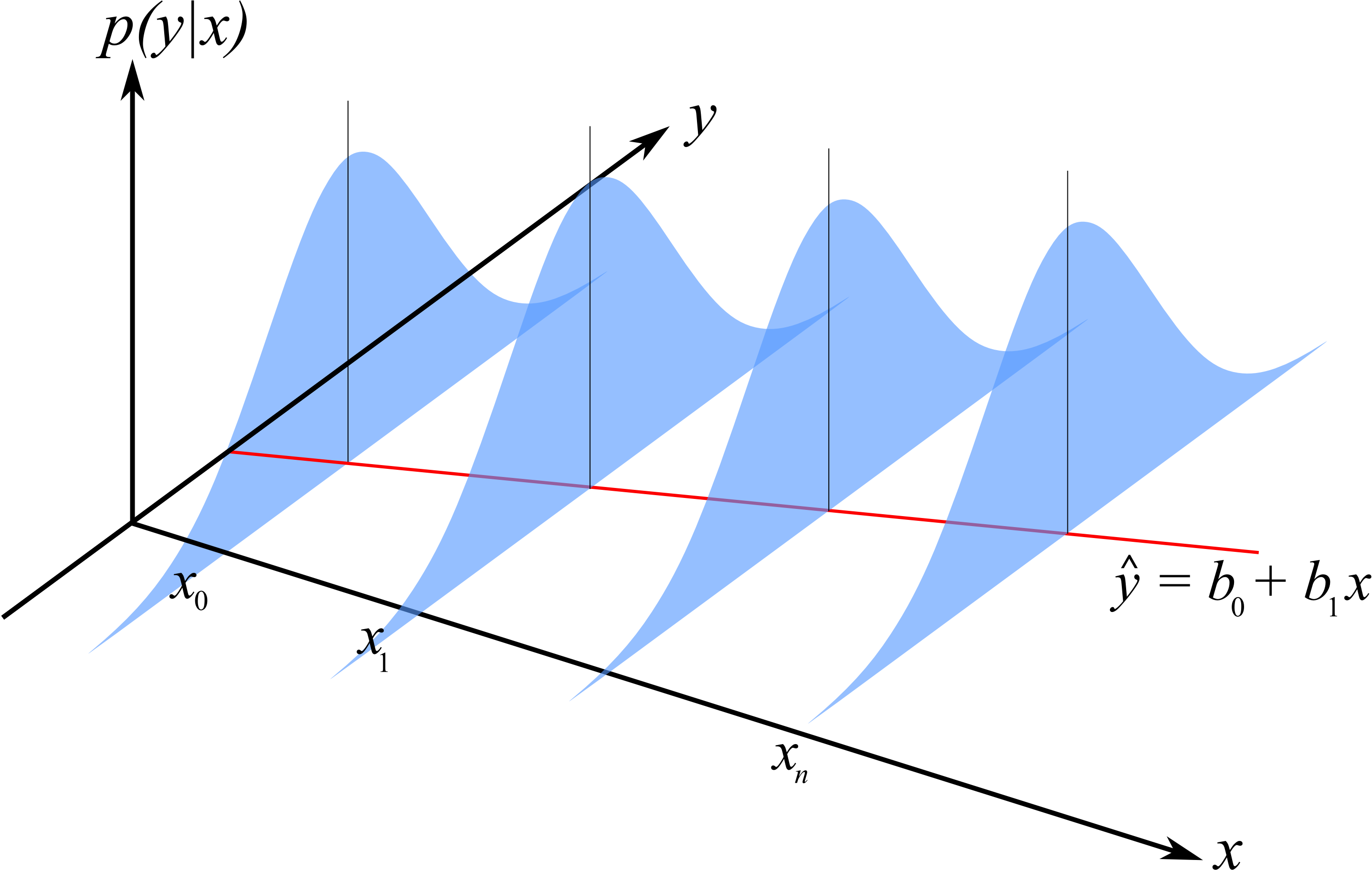
Recall the linear regression model

$$Y_i = \beta_0 + \beta_1 x_i + \epsilon_i,~i=1, \cdots, n,~\textrm{where}~\epsilon_i \sim N(0,\sigma^2).$$

We want to minimize

$$f(\beta_0, \beta_1) = \sum\limits_{i=1}^n e_i^2 = \sum\limits_{i=1}^n(y_i - (\beta_0 + \beta_1x_i))^2.$$

Linear regression model

What is the distribution of $Y_i$?

sum_of_squares = lambda beta, x, y: np.sum((y - beta[0] - beta[1]*x) ** 2)
sum_of_squares([0,0.7], boston.lstat, boston.medv)

184221.366967

However, we have objective of minimizing the sum of squares, so we can pass this function to one of several optimizers in SciPy.

help(fmin)

Help on function fmin in module scipy.optimize.optimize:

fmin(func, x0, args=(), xtol=0.0001, ftol=0.0001, maxiter=None, maxfun=None, full_output=0, disp=1, retall=0, callback=None, initial_simplex=None)
    Minimize a function using the downhill simplex algorithm.
    
    This algorithm only uses function values, not derivatives or second
    derivatives.
    
    Parameters
    ----------
    func : callable func(x,*args)
        The objective function to be minimized.
    x0 : ndarray
        Initial guess.
    args : tuple, optional
        Extra arguments passed to func, i.e., ``f(x,*args)``.
    xtol : float, optional
        Absolute error in xopt between iterations that is acceptable for
        convergence.
    ftol : number, optional
        Absolute error in func(xopt) between iterations that is acceptable for
        convergence.
    maxiter : int, optional
        Maximum number of iterations to perform.
    maxfun : number, optional
        Maximum number of function evaluations to make.
    full_output : bool, optional
        Set to True if fopt and warnflag outputs are desired.
    disp : bool, optional
        Set to True to print convergence messages.
    retall : bool, optional
        Set to True to return list of solutions at each iteration.
    callback : callable, optional
        Called after each iteration, as callback(xk), where xk is the
        current parameter vector.
    initial_simplex : array_like of shape (N + 1, N), optional
        Initial simplex. If given, overrides `x0`.
        ``initial_simplex[j,:]`` should contain the coordinates of
        the jth vertex of the ``N+1`` vertices in the simplex, where
        ``N`` is the dimension.
    
    Returns
    -------
    xopt : ndarray
        Parameter that minimizes function.
    fopt : float
        Value of function at minimum: ``fopt = func(xopt)``.
    iter : int
        Number of iterations performed.
    funcalls : int
        Number of function calls made.
    warnflag : int
        1 : Maximum number of function evaluations made.
        2 : Maximum number of iterations reached.
    allvecs : list
        Solution at each iteration.
    
    See also
    --------
    minimize: Interface to minimization algorithms for multivariate
        functions. See the 'Nelder-Mead' `method` in particular.
    
    Notes
    -----
    Uses a Nelder-Mead simplex algorithm to find the minimum of function of
    one or more variables.
    
    This algorithm has a long history of successful use in applications.
    But it will usually be slower than an algorithm that uses first or
    second derivative information. In practice, it can have poor
    performance in high-dimensional problems and is not robust to
    minimizing complicated functions. Additionally, there currently is no
    complete theory describing when the algorithm will successfully
    converge to the minimum, or how fast it will if it does. Both the ftol and
    xtol criteria must be met for convergence.
    
    Examples
    --------
    >>> def f(x):
    ...     return x**2
    
    >>> from scipy import optimize
    
    >>> minimum = optimize.fmin(f, 1)
    Optimization terminated successfully.
             Current function value: 0.000000
             Iterations: 17
             Function evaluations: 34
    >>> minimum[0]
    -8.8817841970012523e-16
    
    References
    ----------
    .. [1] Nelder, J.A. and Mead, R. (1965), "A simplex method for function
           minimization", The Computer Journal, 7, pp. 308-313
    
    .. [2] Wright, M.H. (1996), "Direct Search Methods: Once Scorned, Now
           Respectable", in Numerical Analysis 1995, Proceedings of the
           1995 Dundee Biennial Conference in Numerical Analysis, D.F.
           Griffiths and G.A. Watson (Eds.), Addison Wesley Longman,
           Harlow, UK, pp. 191-208.

x = boston.lstat
y = boston.medv
b0, b1 = fmin(sum_of_squares, [0,1], (boston.lstat, boston.medv))
b0, b1

Optimization terminated successfully.
         Current function value: 19472.381418
         Iterations: 82
         Function evaluations: 157

(34.55385886222141, -0.9500515380716178)

ax = boston.plot(x='lstat', y='medv', style='o', legend=False, ylabel= 'medv')
ax.plot([0,37], [b0, b0+b1*37])
for xi, yi in zip(x,y):
    ax.plot([xi, xi], [yi, b0+b1*xi], 'k:')

Polynomial regession

We are not restricted to a straight-line regression model; we can represent a curved relationship between our variables by introducing polynomial terms.

sum_squares_quad = lambda beta, x, y: np.sum((y - beta[0] - beta[1]*x - beta[2]*(x**2)) ** 2)
b0,b1,b2 = fmin(sum_squares_quad, [1,1,-1], args=(x,y))
print('\nintercept: {0:.2}, x: {1:.2}, x2: {2:.2}'.format(b0,b1,b2))
ax = boston.plot(x='lstat', y='medv', style='o', legend=False, ylabel = 'medv')
xvals = np.linspace(0, 37, 100)
ax.plot(xvals, b0 + b1*xvals + b2*(xvals**2))

Optimization terminated successfully.
         Current function value: 15347.243159
         Iterations: 187
         Function evaluations: 342

intercept: 4.3e+01, x: -2.3, x2: 0.044

[<matplotlib.lines.Line2D at 0x7fd5ba6a1e80>]

Generalized linear models

Often our data violates one or more of the linear regression assumptions:

• non-linear
• non-normal error distribution
• heteroskedasticity
• this forces us to generalize the regression model in order to account for these characteristics.

As a motivating example, we consider the Olympic medals data.

Linear regression models

• Objective: model the expected value of a continuous variable $Y$, as a linear function of the continuous predictor $X$, $E(Y_i) = \beta_0 + \beta_1X_i$.
• Model structure: $Y_i = \beta_0 + \beta_1X_i + e_i$.
• Model assumptions: $Y$ is is normally distributed, errors are normally distributed, $e_i \sim N(0, \sigma^2)$, and independent, and $X$ is fixed, and constant variance $\sigma^2$.
• Parameter estimates and interpretation: $\hat{\beta}_0$ is estimate of $\beta_0$ or the intercept, and $\hat{\beta}_1$ is estimate of the slope, etc. Think about the interpretation of the intercept and the slope.
• Model fit: $R^2$, residual analysis, F-statistic.
• Model selection: From a plethora of possible predictors, which variables to include?

Generalized linear models (GLM)

• GLM usually refers to conventional linear regression models for a continuous response variable given continuous and/or categorical predictors.
• The form is $y_i \sim N(x^T_i\beta,\sigma^2)$, where $x_i$ contains known covariates and $\beta$ contains the coefficients to be estimated. These models are usually fit by least squares and weighted least squares.
• $y_i$ is assumed to follow an exponential family distribution with mean $\mu_i$, which is assumed to be some (often nonlinear) function of $x^T_i\beta$.

GLM assumptions

• The data $Y_1, Y_2, \cdots, Y_n$ are independently distributed, i.e., cases are independent.
• $Y_i$ does NOT need to be normally distributed, but it typically assumes a distribution from an exponential family (e.g. binomial, Poisson)
• GLM does NOT assume a linear relationship between $Y$ and $X$, but it does assume linear relationship between the transformed response in terms of the link function and the explanatory variables.
• $X$ can be even the power terms or some other nonlinear transformations of the original independent variables.
• Overdispersion (when the observed variance is larger than what the model assumes) maybe present.
• Errors need to be independent but NOT normally distributed.
• It uses MLE rather than OLS.

medals = pd.read_csv('./data/medals.csv')
medals.head()

	medals	population	oecd	log_population
0	1	96165	0	11.473821
1	1	281584	0	12.548186
2	6	2589043	0	14.766799
3	25	10952046	0	16.209037
4	41	18348078	1	16.725035

We expect a positive relationship between population and awarded medals, but the data in their raw form are clearly not amenable to linear regression.

medals.plot(x='population', y='medals', kind='scatter')

<AxesSubplot:xlabel='population', ylabel='medals'>

Part of the issue is the scale of the variables. For example, countries' populations span several orders of magnitude. We can correct this by using the logarithm of population, which we have already calculated.

medals.plot(x='log_population', y='medals', kind='scatter')

<AxesSubplot:xlabel='log_population', ylabel='medals'>

• This is an improvement, but the relationship is still not adequately modeled by least-squares regression.

• This is due to the fact that the response data are counts. As a result, they tend to have characteristic properties.

  • discrete
  • positive
  • variance grows with mean

• To account for this, we can do two things:

  1. model the medal count on the log scale;
  2. assume Poisson, rather than normal.

Poisson regression

• So, we will model the logarithm of the expected value as a linear function of our predictors:

$$y_i \sim \text{Poisson}(\lambda_i)$$ $$\log(\lambda_i) = \eta_i = \beta_0 + \beta_1x_{i,1} + \cdots + \beta_1x_{i,q},$$

• Log link function forces positive mean.

• Poisson log likelihood:

$$\log L = \sum_{i=1}^n -\exp(x_i^T\beta) + y_i (x_i^T \beta)- \log(y_i!)$$

• As we have already done, we just need to code the kernel of this likelihood, and optimize!

# Poisson negative log-likelhood
poisson_loglike = lambda beta, X, y: -(-np.exp(X.dot(beta)) + y*X.dot(beta)).sum()

b1, b0 = fmin(poisson_loglike, [0,1], args=(medals[['log_population']].assign(intercept=1).values, 
                                            medals.medals.values))
b0, b1

Optimization terminated successfully.
         Current function value: -1381.299433
         Iterations: 68
         Function evaluations: 131

(-5.297302917060439, 0.44873025169011005)

ax = medals.plot(x='log_population', y='medals', kind='scatter')
xvals = np.arange(12, 22)
ax.plot(xvals, np.exp(b0 + b1*xvals), 'r--')

[<matplotlib.lines.Line2D at 0x7fd5b8d999a0>]

More on modeling

• Statsmodels for advanced modeling.

• Scikit-learn for statistical learning.