Concepts in text processing
Corpora
Corpus is a large collection of texts. It is a body of written or spoken material upon which a linguistic analysis is based.
A corpus provides grammarians, lexicographers, and other interested parties with better discriptions of a language. Computer-procesable corpora allow linguists to adopt the principle of total accountability, retrieving all the occurrences of a particular word or structure for inspection or randomly selcted samples.
Corpus analysis provide lexical information, morphosyntactic information, semantic information and pragmatic information.
Tokens
A token is the technical name for a sequence of characters, that we want to treat as a group.
The vocabulary of a text is just the set of tokens that it uses, since in a set, all duplicates are collapsed together. In Python we can obtain the vocabulary items with the command:
set().
Stopwords
Stopwords are common words that generally do not contribute to the meaning of a sentence, at least for the purposes of information retrieval and natural language processing.
These are words such as the and a. Most search engines will filter out stopwords from search queries and documents in order to save space in their index.
Stemming
Stemming is a technique to remove affixes from a word, ending up with the stem. For example, the stem of cooking is cook , and a good stemming algorithm knows that the ing suffix can be removed.
Stemming is most commonly used by search engines for indexing words. Instead of storing all forms of a word, a search engine can store only the stems, greatly reducing the size of index while increasing retrieval accuracy.
Frequency Counts
- Frequency Counts the number of hits.
- Frequency counts require finding all the occurences of a particular feature in the corpus.
- So it is implicit in concordancing. Software is used for this purpose. Frequency counts can be explained statistically.
Word Segmenter
Word segmentation is the problem of dividing a string of written language into its component words.
In English and many other languages using some form of the Latin alphabet, the space is a good approximation of a word divider (word delimiter). (Some examples where the space character alone may not be sufficient include contractions like can't for can not.)
However the equivalent to this character is not found in all written scripts, and without it word segmentation is a difficult problem. Languages which do not have a trivial word segmentation process include Chinese, Japanese, where sentences but not words are delimited, Thai and Lao, where phrases and sentences but not words are delimited, and Vietnamese, where syllables but not words are delimited.
Part-Of-Speech Tagger
In corpus linguistics, part-of-speech tagging (POS tagging or POST), also called grammatical tagging or word-category disambiguation, is the process of marking up a word in a text (corpus) as corresponding to a particular part of speech, based on both its definition, as well as its context—i.e. relationship with adjacent and related words in a phrase, sentence, or paragraph.
A simplified form of this is commonly taught to school-age children, in the identification of words as nouns, verbs, adjectives, adverbs, etc.
Named Entity Recognizer
- Named-entity recognition (NER) (also known as entity identification, entity chunking and entity extraction) is a subtask of information extraction that seeks to locate and classify elements in text into pre-defined categories such as the names of persons, organizations, locations, expressions of times, quantities, monetary values, percentages.
Word embeddings
- Word frequency based
- Prediction based
Word embeddings
This is a word embedding for the word “king” (GloVe vector trained on Wikipedia, see here):
[ 0.50451 , 0.68607 , -0.59517 , -0.022801, 0.60046 , -0.13498 , -0.08813 , 0.47377 , -0.61798 , -0.31012 , -0.076666, 1.493 , -0.034189, -0.98173 , 0.68229 , 0.81722 , -0.51874 , -0.31503 , -0.55809 , 0.66421 , 0.1961 , -0.13495 , -0.11476 , -0.30344 , 0.41177 , -2.223 , -1.0756 , -1.0783 , -0.34354 , 0.33505 , 1.9927 , -0.04234 , -0.64319 , 0.71125 , 0.49159 , 0.16754 , 0.34344 , -0.25663 , -0.8523 , 0.1661 , 0.40102 , 1.1685 , -1.0137 , -0.21585 , -0.15155 , 0.78321 , -0.91241 , -1.6106 , -0.64426 , -0.51042 ]
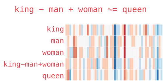
King
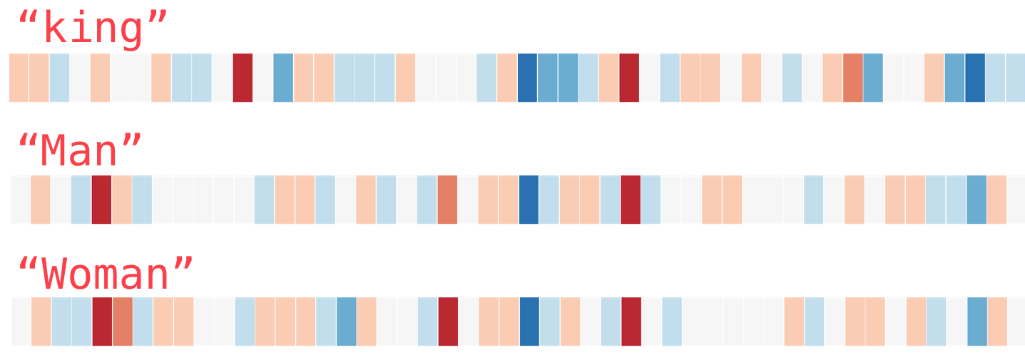

Analogy
Text Feature Extractors
import findspark
findspark.init('/opt/apps/SPARK3/spark-current')
import pyspark
from pyspark.sql import SparkSession
spark = SparkSession.builder.appName("Python Spark with TM").getOrCreate()
Setting default log level to "WARN".
To adjust logging level use sc.setLogLevel(newLevel). For SparkR, use setLogLevel(newLevel).
25/06/02 19:38:04 WARN [Thread-6] Utils: Service 'SparkUI' could not bind on port 4040. Attempting port 4041.
25/06/02 19:38:04 WARN [Thread-6] Client: Neither spark.yarn.jars nor spark.yarn.archive is set, falling back to uploading libraries under SPARK_HOME.
from pyspark.ml.feature import Tokenizer

sentenceData = spark.createDataFrame([
    (0.0, "Hi I heard about Spark"),
    (0.0, "I wish Java could use case classes"),
    (1.0, "Logistic regression models are neat")
], ["label", "sentence"])
tokenizer = Tokenizer(inputCol="sentence", outputCol="words")
tokenizer
Tokenizer_58ff6c9cba3e
wordsData = tokenizer.transform(sentenceData)
wordsData.show()
+-----+--------------------+--------------------+
|label|            sentence|               words|
+-----+--------------------+--------------------+
|  0.0|Hi I heard about ...|[hi, i, heard, ab...|
|  0.0|I wish Java could...|[i, wish, java, c...|
|  1.0|Logistic regressi...|[logistic, regres...|
+-----+--------------------+--------------------+
Count vectorizer
Denote a term by $t$, a document by $d$, and the corpus by $D$. Term frequency $TF(t,d)$ is the number of times that term $t$ appears in document $d$.
# CountVectorizer can be used to get term frequency vectors
from pyspark.ml.feature import CountVectorizer
cv = CountVectorizer(inputCol="words", outputCol="rawFeatures")
model = cv.fit(wordsData)
result = model.transform(wordsData)
result.show(truncate=False)
+-----+-----------------------------------+------------------------------------------+----------------------------------------------------+
|label|sentence                           |words                                     |rawFeatures                                         |
+-----+-----------------------------------+------------------------------------------+----------------------------------------------------+
|0.0  |Hi I heard about Spark             |[hi, i, heard, about, spark]              |(16,[0,8,10,12,13],[1.0,1.0,1.0,1.0,1.0])           |
|0.0  |I wish Java could use case classes |[i, wish, java, could, use, case, classes]|(16,[0,2,3,6,9,11,14],[1.0,1.0,1.0,1.0,1.0,1.0,1.0])|
|1.0  |Logistic regression models are neat|[logistic, regression, models, are, neat] |(16,[1,4,5,7,15],[1.0,1.0,1.0,1.0,1.0])             |
+-----+-----------------------------------+------------------------------------------+----------------------------------------------------+
IDF
- If we only use term frequency to measure the importance, it is very easy to over-emphasize terms that appear very often but carry little information about the document, e.g., “a”, “the”, and “of”. If a term appears very often across the corpus, it means it doesn’t carry special information about a particular document.
- IDF (Inverse document frequency) is a numerical measure of how much information a term provides: $$IDF(t, D) = \log \frac{|D| + 1}{DF(t, D) + 1},$$ where $|D|$ is the total number of documents in the corpus, and document frequency $DF(t,D)$ is the number of documents that contains term $t$.
- Since logarithm is used, if a term appears in all documents, its IDF value becomes 0. Note that a smoothing term is applied to avoid dividing by zero for terms outside the corpus.
IDF
IDFis anEstimatorwhich is fit on a dataset and produces anIDFModel.The
IDFModeltakes feature vectors (generally created fromHashingTForCountVectorizer) and scales each feature.Intuitively, it down-weights features which appear frequently in a corpus.
TF-IDF measure is simply the product of TF and IDF.
from pyspark.ml.feature import HashingTF, IDF
# We use IDF to rescale the feature vectors
idf = IDF(inputCol="rawFeatures", outputCol="features")
idfModel = idf.fit(result)
rescaledData = idfModel.transform(result)
rescaledData.select("label", "features").show(truncate=False)
+-----+--------------------------------------------------------------------------------------------------------------------------------------------------------------+
|label|features                                                                                                                                                      |
+-----+--------------------------------------------------------------------------------------------------------------------------------------------------------------+
|0.0  |(16,[0,8,10,12,13],[0.28768207245178085,0.6931471805599453,0.6931471805599453,0.6931471805599453,0.6931471805599453])                                         |
|0.0  |(16,[0,2,3,6,9,11,14],[0.28768207245178085,0.6931471805599453,0.6931471805599453,0.6931471805599453,0.6931471805599453,0.6931471805599453,0.6931471805599453])|
|1.0  |(16,[1,4,5,7,15],[0.6931471805599453,0.6931471805599453,0.6931471805599453,0.6931471805599453,0.6931471805599453])                                            |
+-----+--------------------------------------------------------------------------------------------------------------------------------------------------------------+
HashingTF
# Alternatively, we can use hashingTF to extract features
from pyspark.ml.feature import HashingTF, IDF
hashingTF = HashingTF(inputCol="words", outputCol="rawFeatures", numFeatures=20)
featurizedData = hashingTF.transform(wordsData)
featurizedData.show(featurizedData.count(), truncate=False)
+-----+-----------------------------------+------------------------------------------+-----------------------------------------------+
|label|sentence                           |words                                     |rawFeatures                                    |
+-----+-----------------------------------+------------------------------------------+-----------------------------------------------+
|0.0  |Hi I heard about Spark             |[hi, i, heard, about, spark]              |(20,[6,8,13,16],[1.0,1.0,1.0,2.0])             |
|0.0  |I wish Java could use case classes |[i, wish, java, could, use, case, classes]|(20,[0,2,7,13,15,16],[1.0,1.0,2.0,1.0,1.0,1.0])|
|1.0  |Logistic regression models are neat|[logistic, regression, models, are, neat] |(20,[3,4,6,11,19],[1.0,1.0,1.0,1.0,1.0])       |
+-----+-----------------------------------+------------------------------------------+-----------------------------------------------+
Word2Vec
Word2Vec is an Estimator which takes sequences of words representing documents and trains a Word2VecModel.
The model maps each word to a unique fixed-size vector.
The Word2VecModel transforms each document into a vector using the average of all words in the document; this vector can then be used as features for prediction, document similarity calculations, etc. Please refer to the MLlib user guide on Word2Vec for more details.
from pyspark.ml.feature import Word2Vec

# Input data: Each row is a bag of words from a sentence or document.
documentDF = spark.createDataFrame([
    ("Hi I heard about Spark".split(" "), ),
    ("I wish Java could use case classes".split(" "), ),
    ("Logistic regression models are neat".split(" "), )
], ["text"])
# Learn a mapping from words to Vectors.
word2Vec = Word2Vec(vectorSize=3, minCount=0, inputCol="text", outputCol="result")
model = word2Vec.fit(documentDF)

result = model.transform(documentDF)
for row in result.collect():
    text, vector = row
    print("Text: [%s] => \nVector: %s\n" % (", ".join(text), str(vector)))
25/05/30 14:14:38 WARN [Executor task launch worker for task 0.0 in stage 24.0 (TID 99)] InstanceBuilder: Failed to load implementation from:dev.ludovic.netlib.blas.JNIBLAS
Text: [Hi, I, heard, about, Spark] =>
Vector: [-0.0879586160182953,0.02657843939960003,-0.06467843998689204]

Text: [I, wish, Java, could, use, case, classes] =>
Vector: [-0.04323068194623504,-0.04786803227450166,0.057834967970848083]

Text: [Logistic, regression, models, are, neat] =>
Vector: [0.01965407431125641,-0.009696281049400568,-0.07410334758460523]
Remove stop words
from pyspark.ml.feature import StopWordsRemover

sentenceData = spark.createDataFrame([
    (0, ["I", "saw", "the", "red", "balloon"]),
    (1, ["Mary", "had", "a", "little", "lamb"])
], ["id", "raw"])

remover = StopWordsRemover(inputCol="raw", outputCol="filtered")
remover.transform(sentenceData).show(truncate=False)
+---+----------------------------+--------------------+
|id |raw                         |filtered            |
+---+----------------------------+--------------------+
|0  |[I, saw, the, red, balloon] |[saw, red, balloon] |
|1  |[Mary, had, a, little, lamb]|[Mary, little, lamb]|
+---+----------------------------+--------------------+
$n$-gram
An $n$-gram is a sequence of $n$ tokens (typically words) for some integer $n$. The
NGramclass can be used to transform input features into $n$-grams.NGramtakes as input a sequence of strings (e.g. the output of aTokenizer).The parameter
nis used to determine the number of terms in each $n$-gram.The output will consist of a sequence of $n$-grams where each $n$-gram is represented by a space-delimited string of $n$ consecutive words. If the input sequence contains fewer than $n$ strings, no output is produced.
from pyspark.ml.feature import NGram

wordDataFrame = spark.createDataFrame([
    (0, ["Hi", "I", "heard", "about", "Spark"]),
    (1, ["I", "wish", "Java", "could", "use", "case", "classes"]),
    (2, ["Logistic", "regression", "models", "are", "neat"]),
    (3, ["I", "like", "regression", "models"]),
], ["id", "words"])

ngram = NGram(n=2, inputCol="words", outputCol="ngrams")

ngramDataFrame = ngram.transform(wordDataFrame)
ngramDataFrame.select("ngrams").show(truncate=False)
+------------------------------------------------------------------+
|ngrams                                                            |
+------------------------------------------------------------------+
|[Hi I, I heard, heard about, about Spark]                         |
|[I wish, wish Java, Java could, could use, use case, case classes]|
|[Logistic regression, regression models, models are, are neat]    |
|[I like, like regression, regression models]                      |
+------------------------------------------------------------------+
Topic modelling with LDA
LDA is an unsupervised method that models documents and topics based on Dirichlet distribution, wherein each document is considered to be a distribution over various topics and each topic is modeled as a distribution over words.
Therefore, given a collection of documents, LDA outputs a set of topics, with each topic being associated with a set of words.
To model the distributions, LDA also requires the number of topics (often denoted by $k$) as an input. For instance, the following are the topics extracted from a random set of tweets from Canadian users where $k = 3$:
- Topic 1: great, day, happy, weekend, tonight, positive experiences
- Topic 2: food, wine, beer, lunch, delicious, dining
- Topic 3: home, real estate, house, tips, mortgage, real estate
from pyspark.ml.clustering import LDA

# Loads data.
dataset = spark.read.format("libsvm").load("file:///opt/apps/SPARK3/spark-3.5.3-hadoop3.2-1.0.0/data/mllib/sample_lda_libsvm_data.txt")
dataset.head(10)
25/05/30 14:14:48 WARN [Thread-6] LibSVMFileFormat: 'numFeatures' option not specified, determining the number of features by going though the input. If you know the number in advance, please specify it via 'numFeatures' option to avoid the extra scan.
[Row(label=0.0, features=SparseVector(11, {0: 1.0, 1: 2.0, 2: 6.0, 4: 2.0, 5: 3.0, 6: 1.0, 7: 1.0, 10: 3.0})),
 Row(label=1.0, features=SparseVector(11, {0: 1.0, 1: 3.0, 3: 1.0, 4: 3.0, 7: 2.0, 10: 1.0})),
 Row(label=2.0, features=SparseVector(11, {0: 1.0, 1: 4.0, 2: 1.0, 5: 4.0, 6: 9.0, 8: 1.0, 9: 2.0})),
 Row(label=3.0, features=SparseVector(11, {0: 2.0, 1: 1.0, 3: 3.0, 6: 5.0, 8: 2.0, 9: 3.0, 10: 9.0})),
 Row(label=4.0, features=SparseVector(11, {0: 3.0, 1: 1.0, 2: 1.0, 3: 9.0, 4: 3.0, 6: 2.0, 9: 1.0, 10: 3.0})),
 Row(label=5.0, features=SparseVector(11, {0: 4.0, 1: 2.0, 3: 3.0, 4: 4.0, 5: 5.0, 6: 1.0, 7: 1.0, 8: 1.0, 9: 4.0})),
 Row(label=6.0, features=SparseVector(11, {0: 2.0, 1: 1.0, 3: 3.0, 6: 5.0, 8: 2.0, 9: 2.0, 10: 9.0})),
 Row(label=7.0, features=SparseVector(11, {0: 1.0, 1: 1.0, 2: 1.0, 3: 9.0, 4: 2.0, 5: 1.0, 6: 2.0, 9: 1.0, 10: 3.0})),
 Row(label=8.0, features=SparseVector(11, {0: 4.0, 1: 4.0, 3: 3.0, 4: 4.0, 5: 2.0, 6: 1.0, 7: 3.0})),
 Row(label=9.0, features=SparseVector(11, {0: 2.0, 1: 8.0, 2: 2.0, 4: 3.0, 6: 2.0, 8: 2.0, 9: 7.0, 10: 2.0}))]
# Trains a LDA model.
lda = LDA(k=10, maxIter=10)
model = lda.fit(dataset)
ll = model.logLikelihood(dataset)
lp = model.logPerplexity(dataset)
print("The lower bound on the log likelihood of the entire corpus: " + str(ll))
print("The upper bound on perplexity: " + str(lp))
The lower bound on the log likelihood of the entire corpus: -817.0874997567644
The upper bound on perplexity: 3.142644229833709
# Describe topics.
topics = model.describeTopics(3)
print("The topics described by their top-weighted terms:")
topics.show(truncate=False)
The topics described by their top-weighted terms:
+-----+-----------+---------------------------------------------------------------+
|topic|termIndices|termWeights                                                    |
+-----+-----------+---------------------------------------------------------------+
|0    |[0, 1, 8]  |[0.10864933036270875, 0.10011127888532786, 0.09713919474835117]|
|1    |[1, 10, 8] |[0.09971340272691882, 0.09635986595981218, 0.09452962012969626]|
|2    |[9, 0, 8]  |[0.10221182795560362, 0.09801672587482077, 0.09536561199948038]|
|3    |[10, 4, 3] |[0.10311849664512139, 0.10220751471589251, 0.09845533560754957]|
|4    |[0, 5, 4]  |[0.15990746929049882, 0.15537240390976645, 0.15247699991605496]|
|5    |[5, 6, 7]  |[0.11586488001195516, 0.1001450522860406, 0.09819014336324963] |
|6    |[10, 6, 3] |[0.21593572362688385, 0.14322851353341437, 0.10835749291798982]|
|7    |[8, 6, 10] |[0.10949954425981283, 0.09791138090693888, 0.09667187416679116]|
|8    |[4, 9, 6]  |[0.10041604448567677, 0.10036848475706113, 0.09788778594781218]|
|9    |[8, 9, 1]  |[0.10393686225665305, 0.10197333879437968, 0.09558884385667736]|
+-----+-----------+---------------------------------------------------------------+
# Shows the result
transformed = model.transform(dataset)
transformed.show(truncate=False)
+-----+---------------------------------------------------------------+--------------------------------------------------------------------------------------------------------------------------------------------------------------------------------------------------------------------+
|label|features                                                       |topicDistribution                                                                                                                                                                                                   |
+-----+---------------------------------------------------------------+--------------------------------------------------------------------------------------------------------------------------------------------------------------------------------------------------------------------+
|0.0  |(11,[0,1,2,4,5,6,7,10],[1.0,2.0,6.0,2.0,3.0,1.0,1.0,3.0])      |[0.004777943110215082,0.004777933453235656,0.004777715229957318,0.004777893603927695,0.4382025535336386,0.00477781392899841,0.5235746226717052,0.004777866150604187,0.004777792948009051,0.0047778653697089285]     |
|1.0  |(11,[0,1,3,4,7,10],[1.0,3.0,1.0,3.0,2.0,1.0])                  |[0.007970921025169244,0.007970957350093975,0.007970885656009523,0.00797099588847754,0.9279545623311699,0.007970836982024915,0.008278548888287458,0.00797081566839799,0.007970702014792795,0.007970774195576699]     |
|2.0  |(11,[0,1,2,5,6,8,9],[1.0,4.0,1.0,4.0,9.0,1.0,2.0])             |[0.004153562579072934,0.004153536645494088,0.004153503286752582,0.004153460734098357,0.44340209421721494,0.0041535744497613125,0.5233696952866023,0.004153536108086881,0.004153562272913015,0.00415347442000355]    |
|3.0  |(11,[0,1,3,6,8,9,10],[2.0,1.0,3.0,5.0,2.0,3.0,9.0])            |[0.0036735687237272456,0.00367355025014438,0.003673569015238193,0.003673535826137115,0.004118984152524214,0.003673546959041967,0.9664926229079428,0.0036735528792876094,0.003673546731524465,0.003673522554432184]  |
|4.0  |(11,[0,1,2,3,4,6,9,10],[3.0,1.0,1.0,9.0,3.0,2.0,1.0,3.0])      |[0.003980198873916475,0.003980202856608425,0.003980187542856114,0.003980214018073737,0.4350498258764531,0.003980201643262402,0.533108719709275,0.00398015292328718,0.0039801679915917295,0.003980128564675886]      |
|5.0  |(11,[0,1,3,4,5,6,7,8,9],[4.0,2.0,3.0,4.0,5.0,1.0,1.0,1.0,4.0]) |[0.003673620839485671,0.0036735847140453035,0.003673603206335511,0.003673585154895501,0.966797123734042,0.003673753576482677,0.003813896800362463,0.0036735802650729246,0.00367367936823112,0.0036735723410468205]  |
|6.0  |(11,[0,1,3,6,8,9,10],[2.0,1.0,3.0,5.0,2.0,2.0,9.0])            |[0.0038206847930207866,0.0038206631423151572,0.003820678718114502,0.003820646195041412,0.004284222979558868,0.0038206634546557334,0.965150488990026,0.003820666845527273,0.0038206552011625437,0.003820629680577797]|
|7.0  |(11,[0,1,2,3,4,5,6,9,10],[1.0,1.0,1.0,9.0,2.0,1.0,2.0,1.0,3.0])|[0.004342545156245695,0.004342570088478088,0.004342537881707782,0.004342583928831243,0.33522219146134913,0.004342584321152026,0.6300374712334958,0.004342509252770688,0.004342524696336219,0.004342481979633276]    |
|8.0  |(11,[0,1,3,4,5,6,7],[4.0,4.0,3.0,4.0,2.0,1.0,3.0])             |[0.004342422221409061,0.004342382555897303,0.004342379127742544,0.004342367439797616,0.9607528017467657,0.004342404699460186,0.004508184484591536,0.004342338519951365,0.004342383959129977,0.004342335245254974]   |
|9.0  |(11,[0,1,2,4,6,8,9,10],[2.0,8.0,2.0,3.0,2.0,2.0,7.0,2.0])      |[0.003293380485104477,0.0032933659218814843,0.0032933287611663477,0.0032933373275839863,0.606159760205621,0.0032932706647909905,0.3674935584619453,0.00329331429094732,0.003293336671463141,0.0032933472094958042]  |
|10.0 |(11,[0,1,2,3,5,6,9,10],[1.0,1.0,1.0,9.0,2.0,2.0,3.0,3.0])      |[0.004153499085151521,0.004153518560893573,0.0041534963390516405,0.004153530366105571,0.2042148767990665,0.004153564542146544,0.7625570959001905,0.004153471155424344,0.004153487226324888,0.0041534600256449734]   |
|11.0 |(11,[0,1,4,5,6,7,9],[4.0,1.0,4.0,5.0,1.0,3.0,1.0])             |[0.004777297184575132,0.004777234349646787,0.004777260476155152,0.004777230148311109,0.9568222668345026,0.004777439753303663,0.004959523703535022,0.004777239011925353,0.00477729464730542,0.0047772138907397075]   |
+-----+---------------------------------------------------------------+--------------------------------------------------------------------------------------------------------------------------------------------------------------------------------------------------------------------+
Topic modeling: Airline review
df = spark.read.csv("/data/Tweets.csv", header=True, inferSchema=True)
df = df.na.drop(subset=["text"])
df.select("airline_sentiment", "text").show(5)
+-----------------+--------------------+
|airline_sentiment|                text|
+-----------------+--------------------+
|          neutral|@VirginAmerica Wh...|
|         positive|@VirginAmerica pl...|
|          neutral|@VirginAmerica I ...|
|         negative|"@VirginAmerica i...|
|         negative|@VirginAmerica an...|
+-----------------+--------------------+
only showing top 5 rows
from pyspark.ml import Pipeline
from pyspark.ml.feature import RegexTokenizer, StopWordsRemover, HashingTF, IDF, StringIndexer
from pyspark.ml.classification import LogisticRegression
from pyspark.ml.evaluation import MulticlassClassificationEvaluator

# 1. 标签编码
label_indexer = StringIndexer(inputCol="airline_sentiment", outputCol="label_index")

# 2. 分词
tokenizer = RegexTokenizer(inputCol="text", outputCol="words", pattern="\\W")

# 3. 去除停用词
remover = StopWordsRemover(inputCol="words", outputCol="filtered_words")

# 4. TF-IDF 特征
hashingTF = HashingTF(inputCol="filtered_words", outputCol="raw_features", numFeatures=20000)
idf = IDF(inputCol="raw_features", outputCol="features")

# 5. 逻辑回归模型(直接设置参数)
lr = LogisticRegression(featuresCol="features", labelCol="label_index", maxIter=50, regParam=0.01, elasticNetParam=0.8)

# 6. 构建 Pipeline
pipeline = Pipeline(stages=[label_indexer, tokenizer, remover, hashingTF, idf, lr])

# 7. 拆分训练/测试集
train_df, test_df = df.randomSplit([0.8, 0.2], seed=42)

# 8. 训练模型
model = pipeline.fit(train_df)

# 9. 预测
predictions = model.transform(test_df)

# 10. 评估准确率
evaluator = MulticlassClassificationEvaluator(
    labelCol="label_index",
    predictionCol="prediction",
    metricName="accuracy"
)
accuracy = evaluator.evaluate(predictions)
print(f"Accuracy = {accuracy:.4f}")
Accuracy = 0.7488
from pyspark.ml import Pipeline
from pyspark.ml.feature import RegexTokenizer, StopWordsRemover, HashingTF, IDF, StringIndexer
from pyspark.ml.classification import LogisticRegression
from pyspark.ml.evaluation import MulticlassClassificationEvaluator
from pyspark.ml.tuning import CrossValidator, ParamGridBuilder

# 1. 标签编码
label_indexer = StringIndexer(inputCol="airline_sentiment", outputCol="label_index")

# 2. 分词(正则化,保留英文单词)
tokenizer = RegexTokenizer(inputCol="text", outputCol="words", pattern="\\W")

# 3. 去除停用词
remover = StopWordsRemover(inputCol="words", outputCol="filtered_words")

# 4. 特征提取:TF-IDF
hashingTF = HashingTF(inputCol="filtered_words", outputCol="raw_features", numFeatures=20000)
idf = IDF(inputCol="raw_features", outputCol="features")

# 5. 逻辑回归模型
lr = LogisticRegression(featuresCol="features", labelCol="label_index", maxIter=50, regParam=0.01, elasticNetParam=0.8)

# 6. 构建 Pipeline
pipeline = Pipeline(stages=[label_indexer, tokenizer, remover, hashingTF, idf, lr])

# 7. 参数网格(在定义了 hashingTF 和 lr 之后)
paramGrid = ParamGridBuilder() \
    .addGrid(hashingTF.numFeatures, [10000, 20000]) \
    .addGrid(lr.regParam, [0.01, 0.1]) \
    .addGrid(lr.elasticNetParam, [0.0, 0.5, 1.0]) \
    .addGrid(lr.maxIter, [20, 50]) \
    .build()

# 8. 模型评估器
evaluator = MulticlassClassificationEvaluator(
    labelCol="label_index",
    predictionCol="prediction",
    metricName="accuracy"
)

# 9. 交叉验证器(确保 pipeline 已定义)
cv = CrossValidator(estimator=pipeline,
                    estimatorParamMaps=paramGrid,
                    evaluator=evaluator,
                    numFolds=3)

# 10. 拆分训练和测试集
train_df, test_df = df.randomSplit([0.8, 0.2], seed=42)

# 11. 拟合模型
cv_model = cv.fit(train_df)

# 12. 预测
predictions = cv_model.transform(test_df)

# 13. 评估准确率
accuracy = evaluator.evaluate(predictions)
print(f"Accuracy = {accuracy:.4f}")
25/06/02 19:48:35 WARN [Thread-6] CacheManager: Asked to cache already cached data.
25/06/02 19:48:35 WARN [Thread-6] CacheManager: Asked to cache already cached data.
Accuracy = 0.7652
# 获取最佳模型(是 PipelineModel)
best_model = cv_model.bestModel

# 获取 Pipeline 中的 stages
stages = best_model.stages

# 最后一阶段是 LogisticRegressionModel
lr_model = stages[-1]

# 打印逻辑回归模型的参数
print("Best LogisticRegression parameters:")
print(f"  - regParam: {lr_model.getRegParam()}")
print(f"  - elasticNetParam: {lr_model.getElasticNetParam()}")
print(f"  - maxIter: {lr_model.getMaxIter()}")

# 如果你也想查看 HashingTF 的参数(比如 numFeatures)
hashingTF_model = stages[3]  # 第4个 stage 是 HashingTF
print("Best HashingTF parameters:")
print(f"  - numFeatures: {hashingTF_model.getNumFeatures()}")
Best LogisticRegression parameters:
  - regParam: 0.01
  - elasticNetParam: 0.5
  - maxIter: 50
Best HashingTF parameters:
  - numFeatures: 20000
spark.stop()