Big Data Essentials
L12: Machine Learning with Spark
Yanfei Kang
yanfeikang@buaa.edu.cn
School of Economics and Management
Beihang University
http://yanfei.site
Machine Learning Library
MLlib is Spark’s machine learning (ML) library. Its goal is to make practical machine learning scalable and easy. At a high level, it provides tools such as:
- ML Algorithms: common learning algorithms such as classification, regression, clustering, and collaborative filtering
- Featurization: feature extraction, transformation, dimensionality reduction, and selection
- Pipelines: tools for constructing, evaluating, and tuning ML Pipelines
- Persistence: saving and load algorithms, models, and Pipelines
- Utilities: linear algebra, statistics, data handling, etc.
MLlib APIs
The RDD-based APIs in the
spark.mllibpackage have entered maintenance mode.The primary Machine Learning API for Spark is now the DataFrame-based API in the
spark.mlpackage.Why the DataFrame-based API?
DataFrames provide a more user-friendly API than RDDs. The many benefits of DataFrames include Spark Datasources, SQL/DataFrame queries, Tungsten and Catalyst optimizations, and uniform APIs across languages.
The DataFrame-based API for MLlib provides a uniform API across ML algorithms and across multiple languages.
DataFrames facilitate practical ML Pipelines, particularly feature transformations. See the Pipelines guide for details.
Start a Spark session
import findspark
findspark.init('/usr/lib/spark-current/')
import pyspark
from pyspark.sql import SparkSession
spark = SparkSession.builder.appName("Python Spark with ML").getOrCreate()
Correlation
Calculating the correlation between two series of data is a common operation in Statistics.
The
spark.mlprovides the flexibility to calculate pairwise correlations among many series. The supported correlation methods are currently Pearson’s and Spearman’s correlation.
from pyspark.ml.linalg import Vectors
from pyspark.ml.stat import Correlation

data = [(Vectors.sparse(4, [(0, 1.0), (3, -2.0)]),),
        (Vectors.dense([4.0, 5.0, 0.0, 3.0]),),
        (Vectors.dense([6.0, 7.0, 0.0, 8.0]),),
        (Vectors.sparse(4, [(0, 9.0), (3, 1.0)]),)]
df = spark.createDataFrame(data, ["features"])

r1 = Correlation.corr(df, "features").head()
print("Pearson correlation matrix:\n" + str(r1[0]))

r2 = Correlation.corr(df, "features", "spearman").head()
print("Spearman correlation matrix:\n" + str(r2[0]))
Summarizer
The
spark.mlprovides vector column summary statistics for Dataframe through Summarizer.Available metrics are the column-wise
max,min,mean,variance, and number ofnonzeros, as well as the totalcount.
sc = spark.sparkContext # make a spark context for RDD
from pyspark.ml.stat import Summarizer
from pyspark.sql import Row
from pyspark.ml.linalg import Vectors

df = sc.parallelize([Row(weight=1.0, features=Vectors.dense(1.0, 1.0, 1.0)),
                     Row(weight=0.0, features=Vectors.dense(1.0, 2.0, 3.0))]).toDF()

# create summarizer for multiple metrics "mean" and "count"
summarizer = Summarizer.metrics("mean", "count")

# compute statistics for multiple metrics with weight
df.select(summarizer.summary(df.features, df.weight)).show(truncate=False)

# compute statistics for multiple metrics without weight
df.select(summarizer.summary(df.features)).show(truncate=False)

# compute statistics for single metric "mean" with weight
df.select(Summarizer.mean(df.features, df.weight)).show(truncate=False)

# compute statistics for single metric "mean" without weight
df.select(Summarizer.mean(df.features)).show(truncate=False)
Machine Learning Pipelines
MLlib standardizes APIs for machine learning algorithms to make it easier to combine multiple algorithms into a single pipeline, or workflow.
The pipeline concept is mostly inspired by the
scikit-learnproject.DataFrame: This ML API uses DataFrame from Spark SQL as an ML dataset, which can hold a variety of data types. E.g., a DataFrame could have different columns storing text, feature vectors, true labels, and predictions.Transformer: A Transformer is an algorithm which can transform one DataFrame into another DataFrame. E.g., an ML model is a Transformer which transforms a DataFrame with features into a DataFrame with predictions.Estimator: An Estimator is an algorithm which can be fit on a DataFrame to produce a Transformer. E.g., a learning algorithm is an Estimator which trains on a DataFrame and produces a model.Pipeline: A Pipeline chains multiple Transformers and Estimators together to specify an ML workflow.Parameter: All Transformers and Estimators now share a common API for specifying parameters.
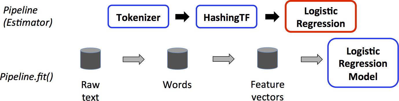
Pipline example: Logistic Regression
from pyspark.ml.linalg import Vectors
from pyspark.ml.classification import LogisticRegression

# Prepare training data from a list of (label, features) tuples.
training = spark.createDataFrame([
    (1.0, Vectors.dense([0.0, 1.1, 0.1])),
    (0.0, Vectors.dense([2.0, 1.0, -1.0])),
    (0.0, Vectors.dense([2.0, 1.3, 1.0])),
    (1.0, Vectors.dense([0.0, 1.2, -0.5]))], ["label", "features"])


# Prepare test data
test = spark.createDataFrame([
    (1.0, Vectors.dense([-1.0, 1.5, 1.3])),
    (0.0, Vectors.dense([3.0, 2.0, -0.1])),
    (1.0, Vectors.dense([0.0, 2.2, -1.5]))], ["label", "features"])
# Create a LogisticRegression instance. This instance is an Estimator.
lr = LogisticRegression(maxIter=10, regParam=0.01)
# Print out the parameters, documentation, and any default values.
print("LogisticRegression parameters:\n" + lr.explainParams() + "\n")
# Learn a LogisticRegression model. This uses the parameters stored in lr.
model1 = lr.fit(training)

# Since model1 is a Model (i.e., a transformer produced by an Estimator),
# we can view the parameters it used during fit().
# This prints the parameter (name: value) pairs, where names are unique IDs for this
# LogisticRegression instance.
print("Model 1 was fit using parameters: ")
print(model1.extractParamMap())
# We may alternatively specify parameters using a Python dictionary as a paramMap
paramMap = {lr.maxIter: 20}
paramMap[lr.maxIter] = 30  # Specify 1 Param, overwriting the original maxIter.
paramMap.update({lr.regParam: 0.1, lr.threshold: 0.55})  # Specify multiple Params.

# You can combine paramMaps, which are python dictionaries.
paramMap2 = {lr.probabilityCol: "myProbability"}  # Change output column name
paramMapCombined = paramMap.copy()
paramMapCombined.update(paramMap2)

# Now learn a new model using the paramMapCombined parameters.
# paramMapCombined overrides all parameters set earlier via lr.set* methods.
model2 = lr.fit(training, paramMapCombined)
print("Model 2 was fit using parameters: ")
print(model2.extractParamMap())
# Make predictions on test data using the Transformer.transform() method.
# LogisticRegression.transform will only use the 'features' column.
# Note that model2.transform() outputs a "myProbability" column instead of the usual
# 'probability' column since we renamed the lr.probabilityCol parameter previously.
prediction = model2.transform(test)
result = prediction.select("features", "label", "myProbability", "prediction") \
    .collect()

for row in result:
    print("features=%s, label=%s -> prob=%s, prediction=%s"
          % (row.features, row.label, row.myProbability, row.prediction))
Pipline example: Decision tree classifier
from pyspark.ml import Pipeline
from pyspark.ml.classification import DecisionTreeClassifier
from pyspark.ml.feature import StringIndexer, VectorIndexer
from pyspark.ml.evaluation import MulticlassClassificationEvaluator

# Load the data stored in LIBSVM format as a DataFrame.
data = spark.read.format("libsvm").load("/opt/apps/ecm/service/spark/2.4.5-hadoop3.1-1.0.2/package/spark-2.4.5-hadoop3.1-1.0.2/data/mllib/sample_libsvm_data.txt")

# Index labels, adding metadata to the label column.
# Fit on whole dataset to include all labels in index.
labelIndexer = StringIndexer(inputCol="label", outputCol="indexedLabel").fit(data)
# Automatically identify categorical features, and index them.
# We specify maxCategories so features with > 4 distinct values are treated as continuous.
featureIndexer =\
    VectorIndexer(inputCol="features", outputCol="indexedFeatures", maxCategories=4).fit(data)

# Split the data into training and test sets (30% held out for testing)
(trainingData, testData) = data.randomSplit([0.7, 0.3])
# Train a DecisionTree model.
dt = DecisionTreeClassifier(labelCol="indexedLabel", featuresCol="indexedFeatures")

# Chain indexers and tree in a Pipeline
pipeline = Pipeline(stages=[labelIndexer, featureIndexer, dt])

# Train model.  This also runs the indexers.
model = pipeline.fit(trainingData)
# Make predictions.
predictions = model.transform(testData)

# Select example rows to display.
predictions.select("prediction", "indexedLabel", "features").show(5)

# Select (prediction, true label) and compute test error
evaluator = MulticlassClassificationEvaluator(
    labelCol="indexedLabel", predictionCol="prediction", metricName="accuracy")
accuracy = evaluator.evaluate(predictions)
print("Test Error = %g " % (1.0 - accuracy))

treeModel = model.stages[2]
# summary only
print(treeModel)
Pipline example: Clustering
from pyspark.ml.clustering import KMeans
from pyspark.ml.evaluation import ClusteringEvaluator

# Loads data.
dataset = spark.read.format("libsvm").load("/opt/apps/ecm/service/spark/2.4.5-hadoop3.1-1.0.2/package/spark-2.4.5-hadoop3.1-1.0.2//data/mllib/sample_kmeans_data.txt")
# Trains a k-means model.
kmeans = KMeans().setK(2).setSeed(1)
model = kmeans.fit(dataset)

# Make predictions
predictions = model.transform(dataset)
# Evaluate clustering by computing Silhouette score
evaluator = ClusteringEvaluator()

silhouette = evaluator.evaluate(predictions)
print("Silhouette with squared euclidean distance = " + str(silhouette))
# Shows the result.
centers = model.clusterCenters()
print("Cluster Centers: ")
for center in centers:
    print(center)
Model Selection with Cross-Validation
from pyspark.ml.classification import LogisticRegression
from pyspark.ml.evaluation import BinaryClassificationEvaluator
from pyspark.ml.feature import HashingTF, Tokenizer
from pyspark.ml.tuning import CrossValidator, ParamGridBuilder

# Prepare training documents, which are labeled.
training = spark.createDataFrame([
    (0, "a b c d e spark", 1.0),
    (1, "b d", 0.0),
    (2, "spark f g h", 1.0),
    (3, "hadoop mapreduce", 0.0),
    (4, "b spark who", 1.0),
    (5, "g d a y", 0.0),
    (6, "spark fly", 1.0),
    (7, "was mapreduce", 0.0),
    (8, "e spark program", 1.0),
    (9, "a e c l", 0.0),
    (10, "spark compile", 1.0),
    (11, "hadoop software", 0.0)
], ["id", "text", "label"])
# Configure an ML pipeline, which consists of tree stages: tokenizer, hashingTF, and lr.
tokenizer = Tokenizer(inputCol="text", outputCol="words")
hashingTF = HashingTF(inputCol=tokenizer.getOutputCol(), outputCol="features")
lr = LogisticRegression(maxIter=10)
pipeline = Pipeline(stages=[tokenizer, hashingTF, lr])
# We now treat the Pipeline as an Estimator, wrapping it in a CrossValidator instance.
# This will allow us to jointly choose parameters for all Pipeline stages.
# A CrossValidator requires an Estimator, a set of Estimator ParamMaps, and an Evaluator.
# We use a ParamGridBuilder to construct a grid of parameters to search over.
# With 3 values for hashingTF.numFeatures and 2 values for lr.regParam,
# this grid will have 3 x 2 = 6 parameter settings for CrossValidator to choose from.
paramGrid = ParamGridBuilder() \
    .addGrid(hashingTF.numFeatures, [10, 100, 1000]) \
    .addGrid(lr.regParam, [0.1, 0.01]) \
    .build()

crossval = CrossValidator(estimator=pipeline,
                          estimatorParamMaps=paramGrid,
                          evaluator=BinaryClassificationEvaluator(),
                          numFolds=2)  # use 3+ folds in practice

# Run cross-validation, and choose the best set of parameters.
cvModel = crossval.fit(training)
# Prepare test documents, which are unlabeled.
test = spark.createDataFrame([
    (4, "spark i j k"),
    (5, "l m n"),
    (6, "mapreduce spark"),
    (7, "apache hadoop")
], ["id", "text"])

# Make predictions on test documents. cvModel uses the best model found (lrModel).
prediction = cvModel.transform(test)
selected = prediction.select("id", "text", "probability", "prediction")
for row in selected.collect():
    print(row)
Lab 7
- Run a logistic regression with airdelay data.