Big Data Essentials
L4: Statistical Modeling with Python
Yanfei Kang
yanfeikang@buaa.edu.cn
School of Economics and Management
Beihang University
http://yanfei.site
Basic python modules for Statistics
NumPy
NumPy is short for Numerical Python, is the foundational package for scientific computing in Python. It contains among other things:
- a powerful N-dimensional array object
- sophisticated (broadcasting) functions
- tools for integrating C/C++ and Fortran code
- useful linear algebra, Fourier transform, and random number capabilities
Readings
SciPy
SciPy is a collection of packages addressing a number of different standard problem domains in scientific computing. Here is a sampling of the packages included:
scipy.integrate: numerical integration routines and differential equation solvers.scipy.linalg: linear algebra routines and matrix decompositions extending beyond those provided innumpy.linalg.scipy.optimize: function optimizers (minimizers) and root finding algorithms.scipy.signal: signal processing tools.scipy.stats: standard continuous and discrete probability distributions (density functions, samplers, continuous distribution functions), various statistical tests, and more descriptive statistics.scipy.cluster: Clustering algorithmsscipy.interpolate: Interpolation and smoothing splinesscipy.ndimage: N-dimensional image processing
Readings
pandas
pandas provides rich data structures and functions designed to make working with structured data fast, easy, and expressive. pandas rounds up the capabilities of Numpy, Scipy and Matplotlib.
- Primary data structures:
SeriesandDataFrame. - Index objects enabling both simple axis indexing and multi-level / hierarchical axis indexing.
- An integrated group by engine for aggregating and transforming data sets.
- Date range generation (date_range) and custom date offsets enabling the implementation of customized frequencies
- Input/Output tools: loading tabular data from flat files (CSV, delimited, Excel 2003), and saving and loading pandas objects from the fast and efficient PyTables/HDF5 format.
- Memory-efficient “sparse” versions of the standard data structures for storing data that is mostly missing or mostly constant (some fixed value).
- Moving window statistics (rolling mean, rolling standard deviation, etc.)
- Static and moving window linear and panel regression.
Readings
Working with Data
Read and write data in Python with stdin and stdout
#! /usr/bin/env python3.8
# line_count.py
import sys
count = 0
data = []
for line in sys.stdin:
    count += 1
    data.append(line)
print(count) # print goes to sys.stdout
print(data)
Then launch a terminal and first make your Python script executable. Then send your file to your Python script
chmod +x line_count.pycat BDE-L3-pyintro.slides.html | ./code/line_count.py
Read from and write to files directly
You can also explicitly read from and write to files directly in your code. Python makes working with files pretty simple.
The first step to working with a text file is to obtain a file object using
open()'r' means read-only
file_for_reading = open('reading_file.txt', 'r')'w' is write -- will destroy the file if it already exists!
file_for_writing = open('writing_file.txt', 'w')'a' is append -- for adding to the end of the file
file_for_appending = open('appending_file.txt', 'a')The second step is do something with the file.
Don't forget to close your files when you're done.
file_for_writing.close()
Note Because it is easy to forget to close your files, you should always use them in a with block, at the end of which they will be closed automatically:
with open(filename,'r') as f:
data = function_that_gets_data_from(f)#! /usr/bin/env python3.8
# hash_check.py
import re
starts_with_hash = 0
# look at each line in the file use a regex to see if it starts with '#' if it does, add 1
# to the count.
with open('./code/line_count.py','r') as file:
for line in file:
if re.match("^#",line):
starts_with_hash += 1
print(starts_with_hash)
Read a CSV file
If your file has no headers, you can use
csv.reader()incsvmodule to iterate over the rows, each of which will be an appropriately split list.If your file has headers, you can either
- skip the header row (with an initial call to
reader.next()), or - get each row as a
dict(with the headers as keys) by usingcsv.DictReader().
- skip the header row (with an initial call to
#! /usr/bin/python3.8


data = []
file = open('data/stocks.csv','r')
next(file)
for line in file:
    data.append(line)

print(data[0])
#! /usr/bin/env python3.8

import csv

data = {'date':[], 'symbol':[], 'closing_price' : []}
with open('data/stocks.csv', 'r') as f:
    reader = csv.DictReader(f, delimiter='\t')
    for row in reader:
        data['date'].append(row["date"])
        data['symbol'].append(row["symbol"])
        data['closing_price'].append(float(row["closing_price"]))
data.keys()
Alternatively, pandas provides read_csv() function to read csv files.
#! /usr/bin/env python3.8

import pandas

data2 = pandas.read_csv('data/stocks.csv', delimiter='\t',header=None)
print(len(data2))
print(type(data2))
The pandas I/O API is a set of top level reader functions accessed like read_csv() that generally return a pandas object. These functions includes
read_excel
read_hdf
read_sql
read_json
read_msgpack (experimental)
read_html
read_gbq (experimental)
read_stata
read_sas
read_clipboard
read_pickle
See pandas IO tools for detailed explanation.
Fitting linear regression models
import numpy as np
import pandas as pd
import matplotlib.pyplot as plt
from scipy.optimize import fmin
import seaborn as sns
# Data available at https://www.kaggle.com/puxama/bostoncsv
# Contains information collected by the U.S Census Service concerning housing in the area of Boston Mass.
boston = pd.read_csv('./data/Boston.csv')
boston.head()
boston.plot(x = 'lstat', y = 'medv', style = 'o', legend=False, ylabel = 'medv')

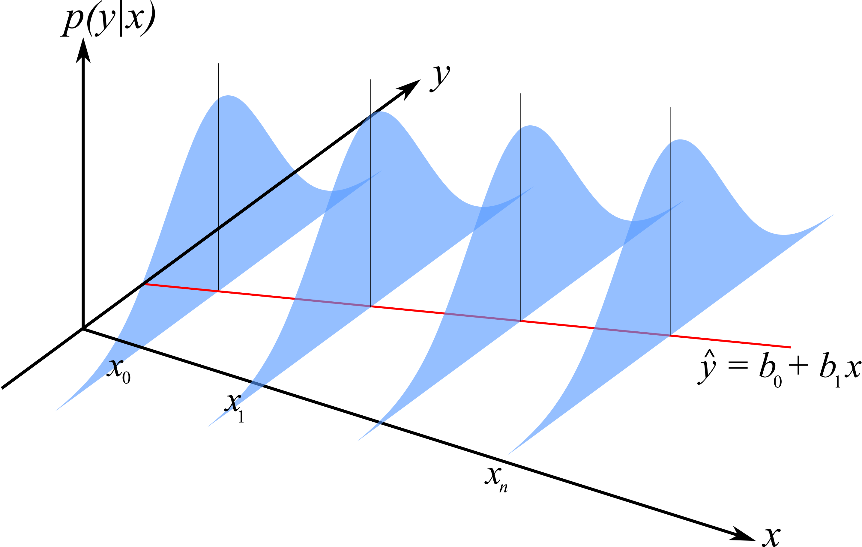
Recall the linear regression model
$$Y_i = \beta_0 + \beta_1 x_i + \epsilon_i,~i=1, \cdots, n,~\textrm{where}~\epsilon_i \sim N(0,\sigma^2).$$We want to minimize
$$f(\beta_0, \beta_1) = \sum\limits_{i=1}^n e_i^2 = \sum\limits_{i=1}^n(y_i - (\beta_0 + \beta_1x_i))^2.$$Linear regression model
What is the distribution of $Y_i$?
sum_of_squares = lambda beta, x, y: np.sum((y - beta[0] - beta[1]*x) ** 2)
sum_of_squares([0,0.7], boston.lstat, boston.medv)
However, we have objective of minimizing the sum of squares, so we can pass this function to one of several optimizers in SciPy.
x = boston.lstat
y = boston.medv
b0, b1 = fmin(sum_of_squares, [0,1], (boston.lstat, boston.medv))
b0, b1
ax = boston.plot(x='lstat', y='medv', style='o', legend=False, ylab = 'medv')
ax.plot([0,37], [b0, b0+b1*37])
for xi, yi in zip(x,y):
    ax.plot([xi]*2, [yi, b0+b1*xi], 'k:')

Polynomial regession
We are not restricted to a straight-line regression model; we can represent a curved relationship between our variables by introducing polynomial terms.
sum_squares_quad = lambda beta, x, y: np.sum((y - beta[0] - beta[1]*x - beta[2]*(x**2)) ** 2)
b0,b1,b2 = fmin(sum_squares_quad, [1,1,-1], args=(x,y))
print('\nintercept: {0:.2}, x: {1:.2}, x2: {2:.2}'.format(b0,b1,b2))
ax = boston.plot(x='lstat', y='medv', style='o', legend=False, ylabel = 'medv')
xvals = np.linspace(0, 37, 100)
ax.plot(xvals, b0 + b1*xvals + b2*(xvals**2))

Generalized linear models
Often our data violates one or more of the linear regression assumptions:
- non-linear
- non-normal error distribution
- heteroskedasticity
- this forces us to generalize the regression model in order to account for these characteristics.
As a motivating example, we consider the Olympic medals data.
Linear regression models
- Objective: model the expected value of a continuous variable $Y$, as a linear function of the continuous predictor $X$, $E(Y_i) = \beta_0 + \beta_1X_i$.
- Model structure: $Y_i = \beta_0 + \beta_1X_i + e_i$.
- Model assumptions: $Y$ is is normally distributed, errors are normally distributed, $e_i \sim N(0, \sigma^2)$, and independent, and $X$ is fixed, and constant variance $\sigma^2$.
- Parameter estimates and interpretation: $\hat{\beta}_0$ is estimate of $\beta_0$ or the intercept, and $\hat{\beta}_1$ is estimate of the slope, etc. Think about the interpretation of the intercept and the slope.
- Model fit: $R^2$, residual analysis, F-statistic.
- Model selection: From a plethora of possible predictors, which variables to include?
Generalized linear models (GLM)
- GLM usually refers to conventional linear regression models for a continuous response variable given continuous and/or categorical predictors.
- The form is $y_i \sim N(x^T_i\beta,\sigma^2)$, where $x_i$ contains known covariates and $\beta$ contains the coefficients to be estimated. These models are usually fit by least squares and weighted least squares.
- $y_i$ is assumed to follow an exponential family distribution with mean $\mu_i$, which is assumed to be some (often nonlinear) function of $x^T_i\beta$.
GLM assumptions
- The data $Y_1, Y_2, \cdots, Y_n$ are independently distributed, i.e., cases are independent.
- $Y_i$ does NOT need to be normally distributed, but it typically assumes a distribution from an exponential family (e.g. binomial, Poisson)
- GLM does NOT assume a linear relationship between $Y$ and $X$, but it does assume linear relationship between the transformed response in terms of the link function and the explanatory variables.
- $X$ can be even the power terms or some other nonlinear transformations of the original independent variables.
- Overdispersion (when the observed variance is larger than what the model assumes) maybe present.
- Errors need to be independent but NOT normally distributed.
- It uses MLE rather than OLS.
medals = pd.read_csv('./data/medals.csv')
medals.head()
We expect a positive relationship between population and awarded medals, but the data in their raw form are clearly not amenable to linear regression.
medals.plot(x='population', y='medals', kind='scatter')

Part of the issue is the scale of the variables. For example, countries' populations span several orders of magnitude. We can correct this by using the logarithm of population, which we have already calculated.
medals.plot(x='log_population', y='medals', kind='scatter')

This is an improvement, but the relationship is still not adequately modeled by least-squares regression.
This is due to the fact that the response data are counts. As a result, they tend to have characteristic properties.
- discrete
- positive
- variance grows with mean
to account for this, we can do two things:
- model the medal count on the log scale;
- assume Poisson errors, rather than normal.
What distribution is in your mind?
Poisson regression
So, we will model the logarithm of the expected value as a linear function of our predictors:
$$\log(\lambda) = X\beta$$In this context, the log function is called a link function. This transformation implies the mean of the Poisson is:
$$\lambda = \exp(X\beta)$$We can plug this into the Poisson likelihood and use maximum likelihood to estimate the regression covariates $\beta$.
$$\log L = \sum_{i=1}^n -\exp(X_i\beta) + Y_i (X_i \beta)- \log(Y_i!)$$As we have already done, we just need to code the kernel of this likelihood, and optimize!
# Poisson negative log-likelhood
poisson_loglike = lambda beta, X, y: -(-np.exp(X.dot(beta)) + y*X.dot(beta)).sum()
b1, b0 = fmin(poisson_loglike, [0,1], args=(medals[['log_population']].assign(intercept=1).values,
                                            medals.medals.values))
b0, b1
ax = medals.plot(x='log_population', y='medals', kind='scatter')
xvals = np.arange(12, 22)
ax.plot(xvals, np.exp(b0 + b1*xvals), 'r--')

Logistic Regression
Fitting a line to the relationship between two variables using the least squares approach is sensible when the variable we are trying to predict is continuous, but what about when the data are dichotomous?
- male/female
- pass/fail
- died/survived
Lab2
Fit a logistic regression to solve a classification problem. You will need
- Likelihood function of logistic regression.
- Optimization.
- Visualization.
You can also make comparisons with packages like scikit-learn or statsmodels.