class: left, bottom, inverse, title-slide # Bayesian Statistics ## Lecture 4: Multiparameter Models ### Yanfei Kang ### 2019/09/18 (updated: 2019-10-10) --- # Introduction - Virtually every practical problem in statistics involves more than one unknown or unobservable quantity. - It is in dealing with such problems that the simple conceptual framework of the Bayesian approach reveals its principal advantages over other methods of inference. - Although a problem can include several parameters of interest, conclusions will often be drawn about one, or only a few, parameters at a time. - In this case, the ultimate aim of a Bayesian analysis is to **obtain the marginal posterior distribution of the particular parameters of interest**. --- # How? - First require the joint posterior distribution of all unknowns. - Then we integrate this distribution over the unknowns that are not of immediate interest to obtain the desired marginal distribution. - Or equivalently, using simulation, we draw samples from the joint posterior distribution and then look at the parameters of interest and ignore the values of the other unknowns. - In many problems there is no interest in making inferences about many of the unknown parameters, although they are required in order to construct a realistic model. Parameters of this kind are often called *nuisance parameters*. --- class: inverse, center, middle # Averaging over ‘nuisance parameters’ --- # Averaging over ‘nuisance parameters’ - Suppose `\(\theta\)` has two parts : `\(\theta = (\theta_1, \theta_2)\)`. - We are only interested in `\(\theta_1\)`. - Then `\(\theta_2\)` is a ‘nuisance’ parameter. --- # Example - `\(y | \mu, \sigma^{2} \sim \mathrm{N}\left(\mu, \sigma^{2}\right).\)` - Interest centers on `\(\mu\)`. - We seek to get `\(p\left(\theta_{1} | y\right).\)` -- - This can be derived from the *joint posterior density:* `$$p\left(\theta_{1}, \theta_{2} | y\right) \propto p\left(y | \theta_{1}, \theta_{2}\right) p\left(\theta_{1}, \theta_{2}\right).$$` - How? --- # How to get `\(p\left(\theta_{1} | y\right)\)`? 1. Average the joint posterier density over `\(\theta_2\)`: `$$p\left(\theta_{1} | y\right)=\int p\left(\theta_{1}, \theta_{2} | y\right) d \theta_{2}.$$` 2. The joint posterior density can be factored to yield: `$$p\left(\theta_{1} | y\right)=\int p\left(\theta_{1} | \theta_{2}, y\right) p\left(\theta_{2} | y\right) d \theta_{2}.$$` - We see a mixture structure. - We see an important practical strategy. --- class: inverse, center, middle # Normal Data with Both Parameters Unknown --- # Normal Data with Both Parameters Unknown - A standard inference problem is to learn about a normal population where both the mean and variance are unknown. - To illustrate Bayesian computation for this problem, suppose we are interested in learning about the distribution of completion times for men between ages 20 and 29 who are running the New York Marathon. - Data: `\(y_1, \cdots, y_{20}\)` in minutes for 20 runners. - They are from `\(N(\mu, \sigma^2)\)`. --- # A noninformative prior distribution `$$g\left(\mu, \sigma^{2}\right) \propto 1 / \sigma^{2}.$$` --- # The joint posterior distribution `$$\begin{aligned} g\left(\mu, \sigma^{2} | y\right) & \propto \sigma^{-n-2} \exp \left(-\frac{1}{2 \sigma^{2}} \sum_{i=1}^{n}\left(y_{i}-\mu\right)^{2}\right) \\ &=\sigma^{-n-2} \exp \left(-\frac{1}{2 \sigma^{2}}\left[\sum_{i=1}^{n}\left(y_{i}-\overline{y}\right)^{2}+n(\overline{y}-\mu)^{2}\right]\right) \\ &=\sigma^{-n-2} \exp \left(-\frac{1}{2 \sigma^{2}}\left[(n-1) s^{2}+n(\overline{y}-\mu)^{2}\right]\right) \end{aligned},$$` where `\(s^{2}=\frac{1}{n-1} \sum_{i=1}^{n}\left(y_{i}-\overline{y}\right)^{2}\)` is the sample variance. **The joint posterior density can be factorized as the product of conditional and marginal posterior densities. How?** --- # The conditional posterior distribution `$$\mu | \sigma^{2}, y \sim \mathrm{N}\left(\overline{y}, \sigma^{2} / n\right).$$` --- # The marginal posterior distribution `$$p\left(\sigma^{2} | y\right) \propto \int \sigma^{-n-2} \exp \left(-\frac{1}{2 \sigma^{2}}\left[(n-1) s^{2}+n(\overline{y}-\mu)^{2}\right]\right) d \mu.$$` `$$\begin{aligned} p\left(\sigma^{2} | y\right) & \propto \sigma^{-n-2} \exp \left(-\frac{1}{2 \sigma^{2}}(n-1) s^{2}\right) \sqrt{2 \pi \sigma^{2} / n} \\ & \propto\left(\sigma^{2}\right)^{-(n+1) / 2} \exp \left(-\frac{(n-1) s^{2}}{2 \sigma^{2}}\right) \end{aligned},$$` which is a scaled inverse- `\(\chi^2\)` density: `\(\sigma^{2} | y \sim \text{Inv-} \chi^2(n-1, s^2).\)` --- # Sampling from the joint posterior distribution 1. First draw `\(\sigma^2\)` from the marginal posterior distribution. 2. Draw `\(\mu\)` from the conditional posterior distribution. --- # Contour plot of the joint posterior density .pull-left[ ```r library(LearnBayes) data(marathontimes) attach(marathontimes) d = mycontour(normchi2post, c(220, 330, 500, 9000), time, xlab="mean",ylab="variance") ``` ] .pull-right[ 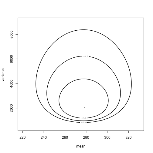<!-- --> ] --- # Simulation .pull-left[ ```r S = sum((time - mean(time))^2) n = length(time) sigma2 = S/rchisq(1000, n - 1) mu = rnorm(1000, mean = mean(time), sd = sqrt(sigma2)/sqrt(n)) d = mycontour(normchi2post, c(220, 330, 500, 9000), time, xlab="mean",ylab="variance") points(mu, sigma2) ``` ] .pull-right[ 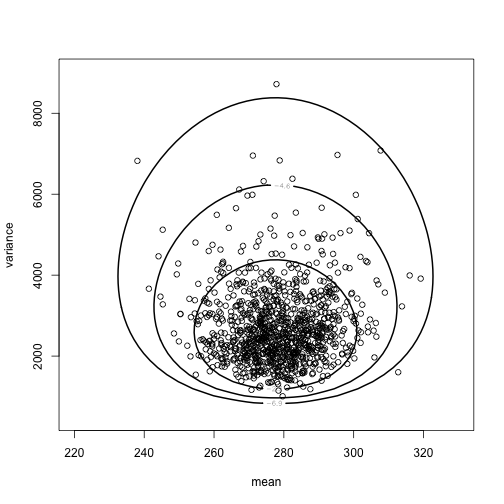<!-- --> ] --- # Inference ```r quantile(mu, c(0.025, 0.975)) ``` ``` ## 2.5% 97.5% ## 256.0856 301.0635 ``` ```r quantile(sqrt(sigma2), c(0.025, 0.975)) ``` ``` ## 2.5% 97.5% ## 38.42701 70.78037 ``` --- # What else can we do to summarize the posterior? ### Do not forget the crude approach: grid approximation - Grid approximation is a very nice way to visualize the posterior (especially for bivariate case). - We can compute `\(g\left(\mu, \sigma^{2} | y\right)\)` for all combinations of `\(\mu\)` and `\(\sigma^2\)`. --- # Grid approximation: create a grid ```r # Data library(LearnBayes) Y <- marathontimes$time n <- length(Y) # Create a grid npts <- 100 mu <- seq( 250, 350,length=npts) s2 <- seq( 30^2,80^2,length=npts) grid_mu <- matrix(mu,npts,npts,byrow=FALSE) grid_s2 <- matrix(s2,npts,npts,byrow=TRUE) ``` --- # Grid approximation: prior .pull-left[ ```r prior <- matrix(1,npts,npts) for(i in 1:n){ prior <- 1/grid_s2 } prior <- prior/sum(prior) library(fields) image.plot(mu,s2,prior,main="Prior") ``` ] .pull-right[ 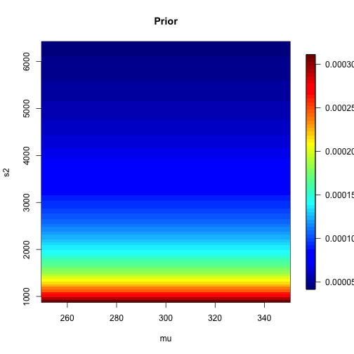<!-- --> ] --- # Grid approximation: likelihood .pull-left[ ```r like <- matrix(1,npts,npts) for(i in 1:n){ like <- like * dnorm(Y[i],grid_mu,sqrt(grid_s2)) } like <- like/sum(like) image.plot(mu,s2,like,main="Likelihood") ``` ] .pull-right[ 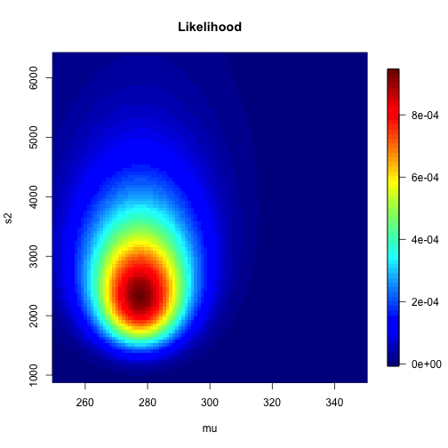<!-- --> ] --- # Grid approximation: posterior .pull-left[ ```r post <- prior * like post <- post/sum(post) image.plot(mu,s2,post,main="Posterior") ``` ] .pull-right[ <!-- --> ] --- # Marginal of `\(\mu\)` .pull-left[ ```r post_mu <-colSums(post) post_mu <- post_mu/sum(post_mu) plot(mu,post_mu,ylab="f(mu|Y)",type="l") abline(v=mean(Y)) ``` ] .pull-right[ <!-- --> ] --- # Marginal of `\(\sigma^2\)` .pull-left[ ```r post_s2 <-rowSums(post) post_s2 <- post_s2/sum(post_s2) plot(s2,post_s2,ylab="f(sigma2|Y)",type="l") abline(v=var(Y)) ``` ] .pull-right[ <!-- --> ] --- # Summarizing the results in a table .pull-left[ ```r post_mean_mu <- sum(mu*post_mu) post_sd_mu <- sum(mu*mu*post_mu) - post_mean_mu^2 post_q025_mu <- max(mu[cumsum(post_mu)<0.025]) post_q975_mu <- max(mu[cumsum(post_mu)<0.975]) post_mean_s2 <- sum(s2*post_s2) post_sd_s2 <- sum(s2*s2*post_s2) - post_mean_s2^2 post_q025_s2 <- max(s2[cumsum(post_s2)<0.025]) post_q975_s2 <- max(s2[cumsum(post_s2)<0.975]) out1 <- c(post_mean_mu,post_sd_mu,post_q025_mu,post_q975_mu) out2 <- c(post_mean_s2,post_sd_s2,post_q025_s2,post_q975_s2) out <- rbind(out1,out2) colnames(out) <- c("Mean","SD","Q025","Q975") rownames(out) <- c("mu","sigma2") knitr::kable(round(out,2), format = 'html') ``` ] .pull-right[ <table> <thead> <tr> <th style="text-align:left;"> </th> <th style="text-align:right;"> Mean </th> <th style="text-align:right;"> SD </th> <th style="text-align:right;"> Q025 </th> <th style="text-align:right;"> Q975 </th> </tr> </thead> <tbody> <tr> <td style="text-align:left;"> mu </td> <td style="text-align:right;"> 282.71 </td> <td style="text-align:right;"> 270.58 </td> <td style="text-align:right;"> 258.08 </td> <td style="text-align:right;"> 322.73 </td> </tr> <tr> <td style="text-align:left;"> sigma2 </td> <td style="text-align:right;"> 2435.52 </td> <td style="text-align:right;"> 380807.48 </td> <td style="text-align:right;"> 1177.78 </td> <td style="text-align:right;"> 3622.22 </td> </tr> </tbody> </table> ] --- # What if we have more than a few parameters? - Integration is difficult. - For most analyses the marginal posteriors will not be a nice distributions. - Grid is not possible either. --- class: inverse, center, middle # No worries! We will come to *Bayesian Computing*.