class: left, bottom, inverse, title-slide # Bayesian Statistics and Computing ## Lecture 11: Bayesian Thinking ### Yanfei Kang ### 2020/03/15 (updated: 2020-03-31) --- # Background - We build models to predict complex phenomena. - We need to make inference to derive estimates of parameters. - Bayesian Statistics allows us to go from data back to probabilistic statements about the parameters. - The procedure relies on Bayes' rule. --- class: inverse, center, middle # Some History of Bayes' Rule By Thomas Bayes (1701–1761) when he solved the problem of 'inverse probability'. 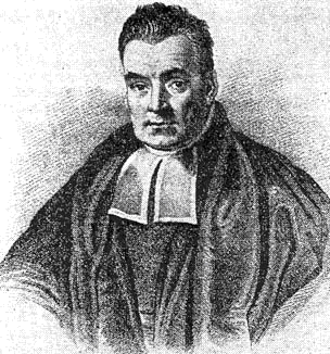 --- class: inverse, center, middle # Some History of Bayes' Rule After Bayes' death, Richard Price published this work in 1763.  --- class: inverse, center, middle # Some History of Bayes' Rule Pioneered and popularised by Pierre-Simon Laplace in 1774, independently.  --- # Bayesian Theories in Machine Learning - The core of machine learning. - Eg1: spell checking. - Eg2: word segmentation. - Eg3: machine translation. - Eg4: spam email filtering. --- class: inverse, center, middle # Bayes' Rule --- # Bayes' Rule .large[ $$ P(A \mid B) = \frac{P(A \,\&\, B)}{P(B)} $$ ] --- # Bayes’ Rule and Diagnostic Testing - Let us consider an example involving the human immunodeficiency virus (HIV). - In the early 1980s, HIV had just been discovered and was rapidly expanding. - False positives (?) and false negatives (?) in HIV testing highly undesirable. --- # Think about probabilities We have the following estimated information: $$ P(\text{ELISA is positive} \mid \text{Person tested has HIV}) = 93\% = 0.93. $$ $$ P(\text{ELISA is negative} \mid \text{Person tested has no HIV}) = 99\% = 0.99. $$ $$ P(\text{Person tested has HIV}) = \frac{1.48}{1000} = 0.00148. $$ What the probability of HIV if ELISA is positive? `$$P(\text{Person tested has HIV} \mid \text{ELISA is positive}) = ?$$` --- # Bayes Learning - One might want to do a second ELISA test after a first one comes up positive. - What is the probability of being HIV positive if the second ELISA test comes back positive? --- # Bayes Learning - The process, of using Bayes' rule to update a probability based on an event affecting it, is called Bayes' updating. - More generally, the what one tries to update can be considered 'prior' information, sometimes simply called the **prior**. - Then, updating this prior using Bayes' rule gives the information conditional on the data, also known as the **posterior**, as in the information after having seen the data. - Going from the prior to the posterior is **Bayes learning** or Bayes updating. --- # Bayesian vs. Frequentist Definitions of Probability - The frequentist definition of probability is based on observation of a large number of trials. The probability for an event `\(E\)` to occur is `\(P(E)\)`, and assume we get `\(n_E\)` successes out of `\(n\)` trials. Then we have $$ P(E) = \lim_{n \rightarrow \infty} \dfrac{n_E}{n}. $$ - On the other hand, the Bayesian definition of probability `\(P(E)\)` reflects our prior beliefs, so `\(P(E)\)` can be any probability distribution. - Think about weather forecasting. --- # Example Based on a 2015 Pew Research poll on 1,500 adults: "We are 95% confident that 60% to 64% of Americans think the federal government does not do enough for middle class people." - There is a 95% chance that this confidence interval includes the true population proportion? - The true population proportion is in this interval 95% of the time? - ? --- # Example - The **Bayesian** alternative is the credible interval, which has a definition that is easier to interpret. - Since a Bayesian is allowed to express uncertainty in terms of probability, a Bayesian credible interval is a range for which the Bayesian thinks that the probability of including the true value is, say, 0.95. - Thus a Bayesian can say that there is a 95% chance that the credible interval contains the true parameter value. --- # Bayesian Inference - Bayesian inference is to modify our beliefs to account for new data. - Before we have data, we have our initial beliefs, which we call prior. - After we have data, we update our beliefs: `$$\text{prior} + \text{data} \rightarrow \text{posterior}.$$` --- # Bayesian Inference via Bayes' Rule .large[ `$$p(\theta|\text{data}) = \frac{p(\text{data}|\theta)p(\theta)}{p(\text{data})}$$` ] --- # How to select prior? - There is no "true" or "correct" prior. - In some cases expert opinion or similar studies can be used to specify an informative prior. - It would be a waste to discard this information - If prior information is unavailable, then the prior should be uninformative. - The prior is best viewed as an initial value to a statistical procedure. --- # How to select prior? - As Bayesian learning continues and more and more data are collected, the posterior concentrates around the true value for any reasonable prior. - However, in a finite sample the prior can have some effect. - Different analysts may pick different priors and thus have different results. --- class: inverse, center, middle # Example --- # Learning About the Proportion of Heavy Sleepers - Suppose a person is interested in learning about the sleeping habits of American college students. - She hears that doctors recommend eight hours of sleep for an average adult. - **What proportion of college students get at least eight hours of sleep?** --- # Learning About the Proportion of Heavy Sleepers Now we reorganize the problem. 1. **Population: ** all American college students. 2. `\(p\)`: the proportion of this population who sleep at least eight hours. 3. Our aim is to learn about the location of `\(p\)`, which is the unknown parameter. --- # Bayesian viewpoint - Use **probability distribution** to describe a person’s beliefs about the uncertainty in `\(p\)`. - This distribution reflects the person’s **subjective prior** opinion about `\(p\)`. - A random sample will be taken. - Before that, research on the sleeping habits to build a prior distribution (e.g. from internet articles or newspaper). - Prior beliefs: `\(p < 0.5\)`, can be any value between 0 and 0.5. --- # Bayesian viewpoint - Suppose our prior density for `\(p\)` is `\(g(p)\)`. - Regard "success" as "sleeping at least 8 hours". - We take a random sample with `\(s\)` successes and `\(f\)` failures. -- - Now we have the likelihood function `$$L(p) \propto p^{s}(1-p)^{f}, 0<p<1.$$` - The posterior for `\(p\)` can be obtained by Bayes' rule: `$$g(p|\text{data}) \propto g(p)L(p).$$` --- # Discrete Prior - List all possible values for `\(p\)` and assign weights for them. - `\(p\)` could be 0.05, 0.15, 0.25, 0.35, 0.45, 0.55, 0.65, 0.75, 0.85, 0.95. - Their weights are 1, 5.2, 8, 7.2, 4.6, 2.1, 0.7, 0.1, 0, 0. --- # Discrete Prior .pull-left[ ```r p = seq(0.05, 0.95, by = 0.1) prior = c(1, 5.2, 8, 7.2, 4.6, 2.1, 0.7, 0.1, 0, 0) prior = prior/sum(prior) plot(p, prior, type = "h", ylab="Prior Probability") ``` ] .pull-right[ <!-- --> ] --- # Likelihood - In our example, 11 of 27 students sleep a sufficient number of hours. - `\(s = 11\)` and `\(f = 16.\)` - Likelihood function: `$$L(p) \propto p^{11}(1-p)^{16}.$$` --- # Posterior .pull-left[ Now compute the posterior probabilities. ```r s <- 11; f <- 16 like <- p^s*(1-p)^f # calculate likelihood post <- prior*like post <- post/sum(post) par(mfrow=c(2,1)) plot(p,prior,type = "h",lty = 2,ylim = c(0,1),ylab = "prior") plot(p,post,type = "h",lty = 1,ylim = c(0,1),ylab = "posterior") ``` ] .pull-right[ <!-- --> ] --- # Beta Prior - `\(p\)` is a continuous parameter. - Alternative is to construct a density `\(g(p)\)` on [0, 1]. - Suppose she believes that the proportion is equally likely to be smaller or larger than `\(p = 0.3\)`. - And she is 90% confident that `\(p\)` is less than 0.5. - A convenient family of densities for a proportion is `$$g(p) \propto p^{a-1}(1-p)^{b-1}, 0<p<1.$$` - **How to select `\(a\)` and `\(b\)`?** --- # Beta Prior - Here the person believes that the median and 90th percentiles of the proportion are given, respectively, by 0.3 and 0.5. - ` beta.select()` in R can find the shape parameters of the beta density that match this prior knowledge. ```r quantile2=list(p=.9,x=.5) quantile1=list(p=.5,x=.3) LearnBayes::beta.select(quantile1,quantile2) ``` ``` ## [1] 3.26 7.19 ``` --- # Posterior - Combining this beta prior with the likelihood function, one can show that the posterior density is also of the beta form with updated parameters `\(a + s\)` and `\(b + f\)`. `$$g(p | \text { data }) \propto p^{a+s-1}(1-p)^{b+f-1}, 0<p<1.$$` - This is an example of a **conjugate** analysis, where the prior and posterior densities have the same functional form. - The prior, likelihood, and posterior are all in the beta family. --- # Posterior .pull-left[ ```r # Plot beta prior, likelihood and posterior a = 3.26; b = 7.19; s = 11; f = 16 *curve(dbeta(x,a+s,b+f), from=0, to=1, * xlab="p",ylab="Density",lty=1,lwd=4) curve(dbeta(x,s+1,f+1),add=TRUE,lty=2,lwd=4) curve(dbeta(x,a,b),add=TRUE,lty=3,lwd=4) legend(.7,4,c("Prior","Likelihood","Posterior"), lty=c(3,2,1),lwd=c(3,3,3)) ``` ] .pull-right[ <!-- --> ] --- # Making Inferences via Posterior **1. Is it likely that the proportion of heavy sleepers is greater than 0.5?** **2. What is the 90% interval estimate for `\(p\)`?** ??? ```r # Exact inferences 1 - pbeta(0.5, a + s, b + f) ``` ``` ## [1] 0.0690226 ``` ```r qbeta(c(0.05, 0.95), a + s, b + f) ``` ``` ## [1] 0.2555267 0.5133608 ``` ```r # Inferences based on simulation ps = rbeta(1000, a + s, b + f) hist(ps,xlab="p",main="") ``` <!-- --> ```r sum(ps >= 0.5)/1000 ``` ``` ## [1] 0.076 ``` ```r quantile(ps, c(0.05, 0.95)) ``` ``` ## 5% 95% ## 0.2485545 0.5153966 ``` --- class: inverse, center, middle # Example --- # Normal Distribution with Known Mean but Unknown Variance - We estimate an unknown variance using American football scores. - The focus is on the difference `\(d\)` between a game outcome (winning score minus losing score) and a published point spread. - We have observations: `\(d_1, d_2, \cdots, d_n\)`. - We assume they are normally distributed with mean 0 and variance `\(\sigma^2\)`. --- # ### Likelihood function `$$L\left(\sigma^{2}\right) \propto\left(\sigma^{2}\right)^{-n / 2} \exp \left\{-\sum_{i=1}^{n} d_{i}^{2} /\left(2 \sigma^{2}\right)\right\}, \sigma^{2}>0.$$` -- ### Prior We use the noninformative prior `$$p\left(\sigma^{2}\right) \propto 1 / \sigma^{2}.$$` -- ### Posterior `$$g\left(\sigma^{2} | \text { data }\right) \propto\left(\sigma^{2}\right)^{-n / 2-1} \exp \left\{-v /\left(2 \sigma^{2}\right)\right\},$$` where `\(v=\sum_{i=1}^{n} d_{i}^{2}.\)` --- # Now if we define precision parameter `\(P=1 / \sigma^{2},\)` 1. **What is the distribution of `\(P\)`?** 2. **What is the point estimate and a 95% probability interval for the standard deviation `\(\sigma\)`?** ??? - If `\(X\)` is distributed with density `\(f(x)\)`, then the density of `\(y = 1/x\)` is `\(g(y)=\frac{1}{y^{2}} f\left(\frac{1}{y}\right)\)`. - `\(P\)` is distributed as `\(U/v\)`. - `\(U\)` has a `\(\chi^2\)` distribution with `\(n\)` degrees of freedom. --- # Normal Dis. with Known Mean but Unknown Variance .pull-left[ Data available [here](https://yanfei.site/docs/bsc/footballscores.txt). ```r # Football scores from 672 professional American football games. d = read.table('footballscores.txt', header = TRUE)$scores n = length(d); v = sum(d^2) # simulate from posterior *P = rchisq(1000, n)/v s = sqrt(1/P) quantile(s, probs = c(0.025, 0.5, 0.975)) hist(s,main="") ``` ] .pull-right[ ``` ## 2.5% 50% 97.5% ## 13.14580 13.81775 14.55710 ``` <!-- --> ] --- class: inverse, center, middle # Everything boils down to summarizing the posterior. -- #### 1. Simulate from R. -- #### 2. Brute-force. -- #### 3. Deterministic tools. -- #### 4. Computing (more general). --- # Summary - Bayesian rule. - Bayesian reference. - Difference with Frequentist. - Priors. - Everything boils down to summarizing the posterior. - Examples. --- # References and further readings ### References - Sections 2.1, 2.2, 2.3 and 2.5 of BDA book by Gelman et.al. - Chapter 1 of [An Introduction to Bayesian Thinking](https://statswithr.github.io/book/the-basics-of-bayesian-statistics.html). ### Further readings - Section 2.8 for noninformative priors. - Section 3.2 for normal distribution with `\(\mu\)` and `\(sigma\)` both unknown.