Bayesian Statistics and Computing

class: left, bottom, inverse, title-slide

# Bayesian Statistics and Computing
## Lecture 14: Markov chain Monte Carlo (MCMC) Methods
### Yanfei Kang
### 2020/03/15 (updated: 2020-04-09)

---

# Limitations of independent Monte Carlo methods

- The ability to sample from the posterior distribution is essential to the practice of Bayesian statistics.

- Direct sampling
    - Sometimes difficult to find the inverse function.

- Rejection sampling and importance sampling 
    - Doesn’t work well if proposal is very different from the target.
    - Yet constructing a proposal similar to the target can be difficult.

- Intuition of MCMC
    - Instead of a fixed proposal, use an adaptive proposal.
    
---
class: inverse, center, middle
# Markov chain

---
# What is Markov chain?

A *Markov chain* is a sequence of random variables `$\theta^1, \theta^2, \cdots,$` for which, for any `$t$`, the distribution of `$\theta^t$` given all previous `$\theta$`'s depends only the most recent value, `$\theta^{t-1}$`.

---
# The key to MCMC's success

- Not the Markov property.

- But the approximate distributions are improved at each step in simulation (in the sense of converging to the target distribution).

---
class: inverse, center, middle
# The Metropolis algorithm

---
# The Metropolis algorithm

- The Metropolis algorithm was developed in a 1953 paper by Metropolis, Rosenbluth, Rosenbluth, Teller and Teller.

- The aim is to simulate `$x \sim p(x)$` where `$p(x)$` is called the target density.

- We will need a proposal density `$q\left(x^{[\text {new}]} | x^{[\text {old }]} \right).$`

- For example one choice of `$q$` is `$$x^{[\mathrm{new}]} \sim N\left(x^{[\mathrm{old}]}, 1\right).$$`

- This is called a Random Walk proposal.

---
# Symmetric proposal

- An important property of `$q$` in the Metropolis algorithm is symmetry of the proposal `$$q\left(x^{[\text {new}]} | x^{[\text {old}]}\right)=q\left(x^{[\text {old}]} | x^{[\text {new}]} \right).$$`

- Can you confirm this is true?

---
# Accept and reject

To make sure this Markov chain converges to our target, we need to include the following.

1. At step `$i+1$`, set `$x^{[\mathrm{old}]} = x^{[i]}$`.
2. Generate `$x^{[\mathrm{new}]} \sim N\left(x^{[\mathrm{old}]}, 1\right)$`, and compute `$$\alpha=\min \left(1, \frac{p\left(x^{[\mathrm{new}]}\right)}{p\left(x^{[\mathrm{old}]}\right)}\right).$$`
3. Set `$x^{[i+1]} = x^{[\mathrm{new}]}$` with probability `$\alpha$` (accept); set `$x^{[i+1]} = x^{[\mathrm{old}]}$` with probability `$1-\alpha$` (reject).

---
# Example

.pull-left[
Here is a target distribution to sample from. It’s the weighted sum of two normal distributions. Sample using the Metropolis algorithm, and plot the trace.

```r
p <- 0.4
mu <- c(-1, 2)
sd <- c(0.5, 2)
f <- function(x) {
    p * dnorm(x, mu[1], sd[1]) + (1 - p) * dnorm(x, mu[2], sd[2])
}
curve(f(x), -4, 8, n = 301, las = 1)
```
]

.pull-right[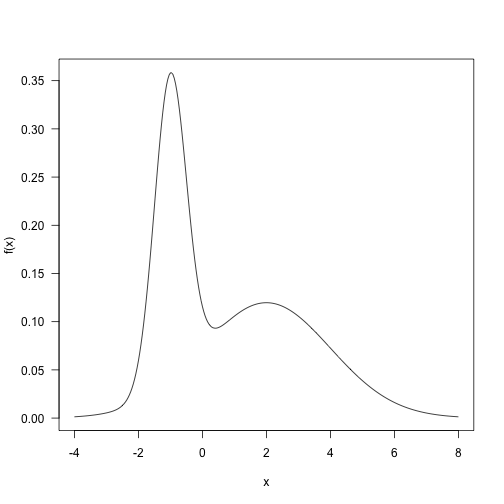
![](BSC-L14-MCMC_files/figure-html/unnamed-chunk-1-1.png)
]

---
#

### Define `$q$`

```r
q <- function(x) rnorm(1, x, 4)
```

### Define the step

```r
step <- function(x, f, q) {
  ## Pick new point
  xp <- q(x)
  ## Acceptance probability:
  alpha <- min(1, f(xp) / f(x))
  ## Accept new point with probability alpha:
  if (runif(1) < alpha)
    x <- xp
  ## Returning the point:
  x
}
```

---
#  Let's run it

```r
run <- function(x, f, q, nsteps) {
  res <- matrix(NA, nsteps, length(x))
  for (i in seq_len(nsteps))
    res[i,] <- x <- step(x, f, q)
  return(res)
}
res <- run(-10, f, q, 1100)
```

---
# Trace plot (1100 samples, with the first 100 burn-in)

---
# Does it resembles our target?

.pull-left[

```r
hist(res[101:1100], 50, freq=FALSE, main="", ylim=c(0, .4), las=1,
     xlab="x", ylab="Probability density")
z <- integrate(f, -Inf, Inf)$value
curve(f(x) / z, add=TRUE, col="red", n=200)
```
]

.pull-right[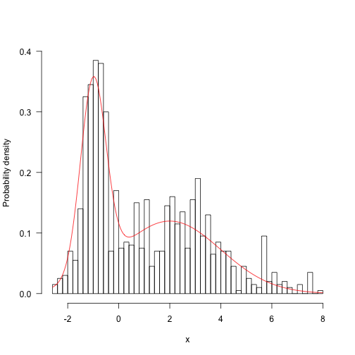
![](BSC-L14-MCMC_files/figure-html/unnamed-chunk-6-1.png)
]

---
# Exercise

1. Try 10000 samples.

2. Try different initial values (even very unrealistic ones).

3. Try different values of standard deviation for `$q$` (e.g., 50, 0.1). Plot their trace plots together with the previous one. Calculate their acceptance rates. Your findings?

4. Based on 3, plot the autocorrelation plots of the three traces. Your findings?

---
# Findings

- For a random walk proposal it is not good to have an acceptance rate that is too high or too low.

- What exactly is too high and too low?

- It depends on many things including the target and proposal.

- A rough rule is to aim for an acceptance rate between 20% and 70%.

- If your acceptance rate is outside this range the proposal variance can be doubled or halved.

---
# Findings

- It is better to have lower correlation in the Markov chain.

- The efficiency of the chain can be measured using the effective sample size.

- The effective sample size can be computed using the function `effectiveSize` in the R Package **coda**.

- Obtain an effective sample size for your samples.

---
class: inverse, center, middle
# The Metropolis Hastings algorithm

---
# The Metropolis Hastings algorithm

1. At step `$i+1$`, set `$x^{[\mathrm{old}]} = x^{[i]}$`.
2. Simulate `$x^{[\mathrm{new}]}$` from the proposal density `$q\left(x^{[\mathrm{new}]}|x^{[\mathrm{old}]}\right)$`, and compute `$$\alpha=\min \left(1, \frac{p\left(x^{[\mathrm{new}]}\right) q\left(x^{[\mathrm{old}]}|x^{[\mathrm{new}]}\right)}{p\left(x^{[\mathrm{old}]}\right) q\left(x^{[\mathrm{new}]}|x^{[\mathrm{old}]}\right)}\right).$$`
3. Set `$x^{[i+1]} = x^{[\mathrm{new}]}$` with probability `$\alpha$` (accept); set `$x^{[i+1]} = x^{[\mathrm{old}]}$` with probability `$1-\alpha$` (reject).

---
# Choices for the Metropolis Hastings algorithm

- Random walk Metropolis Hastings

`$x^{[\mathrm{new}]} = x^{[\mathrm{old}]} + \epsilon$`, where `$\epsilon \sim g$` and `$g$` is a probability density symmetric about 0. In this case  `$q\left(x^{[\mathrm{new}]}|x^{[\mathrm{old}]}\right) = q\left(x^{[\mathrm{old}]}|x^{[\mathrm{new}]}\right)$`.

- Independent Metropolis Hastings

`$q\left(x^{[\mathrm{new}]}|x^{[\mathrm{old}]}\right) = q\left(x^{[\mathrm{new}]}\right)$`, and `$q\left(x^{[\mathrm{old}]}|x^{[\mathrm{new}]}\right) = q\left(x^{[\mathrm{old}]}\right)$`.

---
# 2d example

This is a function that makes a multivariate normal density given a vector of means and variance-covariance matrix.

```r
make.mvn <- function(mean, vcv) {
  logdet <- as.numeric(determinant(vcv, TRUE)$modulus)
  tmp <- length(mean) * log(2 * pi) + logdet
  vcv.i <- solve(vcv)

function(x) {
    dx <- x - mean
    exp(-(tmp + rowSums((dx %*% vcv.i) * dx))/2)
  }
}
```

---
# Target density

.pull-left[

```r
mu1 <- c(-1, 1)
mu2 <- c(2, -2)
vcv1 <- matrix(c(1, .25, .25, 1.5), 2, 2)
vcv2 <- matrix(c(2, -.5, -.5, 2), 2, 2)
f1 <- make.mvn(mu1, vcv1)
f2 <- make.mvn(mu2, vcv2)
f <- function(x)
    f1(x) + f2(x)

x <- seq(-5, 6, length=71)
y <- seq(-7, 6, length=61)
xy <- expand.grid(x=x, y=y)
z <- matrix(apply(as.matrix(xy), 1, f), length(x), length(y))

image(x, y, z, las=1)
contour(x, y, z, add=TRUE)
```
]

.pull-right[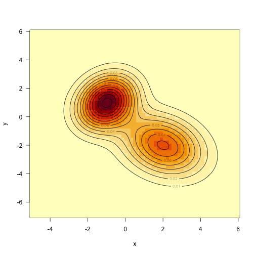
![](BSC-L14-MCMC_files/figure-html/unnamed-chunk-8-1.png)
]

---
# Metropolis sampling

.pull-left[

```r
q <- function(x, d=8)
    x + runif(length(x), -d/2, d/2)

x0 <- c(-4, -4)
set.seed(1)
samples <- run(x0, f, q, 1000)

image(x, y, z, xlim=range(x, samples[,1]), ylim=range(x, samples[,2]))
contour(x, y, z, add=TRUE)
lines(samples[,1], samples[,2], col="#00000088")
```
]

.pull-right[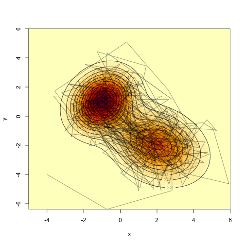
![](BSC-L14-MCMC_files/figure-html/unnamed-chunk-9-1.png)
]

---
# More samples

.pull-left[

```r
samples <- run(x0, f, q, 100000)
smoothScatter(samples)
contour(x, y, z, add=TRUE)
```
]

.pull-right[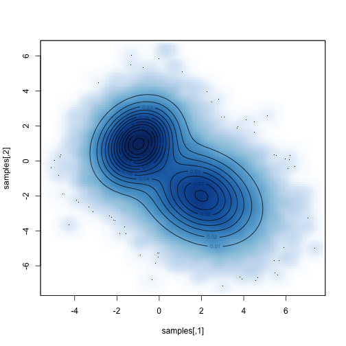
![](BSC-L14-MCMC_files/figure-html/unnamed-chunk-10-1.png)
]

---
# Indirect method v.s. Metropolis Hastings

- Some similarities
    - Both require a proposal.
    - Both are more efficient when the proposal is a good approximation to the target.
    - Both involve some form of accepting/rejecting.

- Some differences
    -  Indirect method produces an independent sample, MH samples are correlated. 
    - Indirect method requires `$p(x)/q(x)$` to be finite for all `$x$`.
    - MH works better when `$x$` is a high-dimensional vector.

---
class: inverse, center, middle
# Gibbs sampler

---
# Gibbs sampler

- The standard Metropolis algorithm updates the entire parameter vector at once with a single step. Hence, a `$p$`-dimensional parameter vector must have a  `$p$`-dimensional proposal distribution  `$q$`.

- The beauty of Gibbs sampling is that it simplifies a complex high-dimensional problem by breaking it down into simple, low-dimensional problems.

---
# Gibbs sampler

- This gives the Gibbs Sampler. If our current state is `$(x^{[i]}, y^{[i]})$`, then we update our parameter values with the following steps.
    1. Generate `$x^{[i+1]} \sim p\left(x|y^{[i]}\right).$`
    2. Generate `$y^{[i+1]} \sim p\left(y|x^{[i+1]}\right).$`
    
- `$x$` and `$y$` can be swapped around.

- It works for more than two variables (think about the case with three parameters).

- Always make sure the conditioning variables are at the most recent state.

---
# Gibbs sampler

- If it is easy to simulate from the conditional distribution `$f(x|y)$` then that can be used as a proposal.

- What is the acceptance ratio?

`$$\begin{aligned} \alpha &= \mathrm{min} \left(1, \frac{p\left(x^{[i+1]}, y\right) p\left(x^{[i]} | y\right)}{p\left(x^{[i]}, y\right) p\left(x^{[i+1]} | y\right)}\right) \\ &= \mathrm{min} \left(1, \frac{p(x^{[i+1]} | y) p(y) p\left(x^{[i]} | y\right)}{p(x^{ [i]}| y) p(y) p(x^{[i+1]} | y)}\right) \\ &=1.\end{aligned}$$`

---
# Gibbs sampler

- Advantages of Gibbs sampling
    - No need to tune proposal distribution.
    - Proposals are always accepted.

- Disadvantages of Gibbs sampling
    - Need to be able to derive conditional probability distributions.
    - Need to be able to (cheaply) draw random samples from conditional probability distributions.
    - Can be very slow if parameters are correlated because you cannot take "diagonal" steps.

---
# Metropolis within Gibbs

- Even if the individual conditional distributions are not easy to simulate from, Metropolis Hastings can be used within each Gibbs step.

- This works very well because it breaks down a multivariate problem into smaller univariate problems.

- We will practice some of these algorithms in the context of Bayesian Inference.

---
class: inverse, center, middle
# The Bayesian linear regression model

---
# Linear regression

- Recall the linear regression model

`$$y_i = \beta_0 + \beta_1 x_1 + ... + \beta_p x_p + \epsilon_i,$$`
    where `$\epsilon_i \sim N(0, \sigma^2).$`

- We are intertested in the joint distribution of
    `$\beta_0,\beta_1,...\beta_p$` and `$\sigma^2$`.

- You know how to get that by OLS under the Gaussian assumption. We have
    `$\beta|\sigma^2 \sim N\left[(x'x)^{-1}x'y,(x'x)^{-1}\sigma^2\right]$` and `$\sigma^2 \sim \chi^2(n-p)$`.
    
---
# The Bayesian approach

- We know by the Bayes' rule `$$\begin{aligned} p\left(\beta, \sigma^{2} | y, x\right) & \propto p\left(y | \beta, \sigma^{2}, x\right) p\left(\beta, \sigma^{2}\right) \\ &=p\left(y | \beta, \sigma^{2}, x\right) p\left(\beta | \sigma^{2}\right) p\left(\sigma^{2}\right) \end{aligned}$$`
                              
      where `$p(y|\beta,\sigma^2,x)$` is the **likelihood** for the
      model and `$p(\beta,\sigma^2) = p(\beta|\sigma^2)p(\sigma^2)$` is
      the **prior** information of the parameters and
      `$p(\beta,\sigma^2|y,x)$` is called the **posterior**.

- **The Bayesian way**: Let's just draw random samples
      from `$p(\beta,\sigma^2|y,x)$`.

---
# Sampling the Posterior

- Write down the likelihood function.
- Specify the prior.
- Write down the posterior.
- Use Gibbs to draw. Set a initial value for `$\beta^{(0)}$` and `$\sigma^{2(0)}$`.
    - Draw a random vector `$\beta^{(1)}$` from `$p(\beta^{(1)} | \sigma^{2(0)},y,x)$`
    - Draw a random number `$\sigma^{2(1)}$` from `$p(\sigma^{2(1)}| \beta^{(1)} ,y,x)$`
    - Draw a random vector `$\beta^{(2)}$` from `$p(\beta^{(2)} | \sigma^{2(1)},y,x)$`
    - Draw a random number `$\sigma^{2(2)}$` from `$p(\sigma^{2(2)}| \beta^{(2)} ,y,x)$`
    - Draw a random vector `$\beta^{(3)}$` from `$p(\beta^{(3)} | \sigma^{2(2)},y,x)$`
    - Draw a random number `$\sigma^{(3)}$` from `$p(\sigma^{2(3)}| \beta^{(3)} ,y,x)$`
    - ...
    - ...
- Summarize `$\beta^{(1)},\beta^{(2)},...,\beta^{(n)}$`
- Summarize `$\sigma^{(1)},\sigma^{(2)},...,\sigma^{(n)}$`

---
# Lab 11

Work on  Metroplis within Gibbs for linear regression on the `bodyfat` data you used for SGD.

- Priors for `$\beta$` and `$\sigma^2$` (e.g., `$\beta \sim N(0, I)$` and `$\sigma^2 \sim \chi^2(10)$`).

- Write down the likelihood.

- Write down the posterior.

- Go to Gibbs.

- Use random walk proposal for Metropolis.

- Summary your samples.

---
# Lab 11 hints

```r
## Generate data for linear regression
n <- 1000
p <- 3
epsilon <- rnorm(n, 0, 0.1)
beta <- matrix(c(-3, 1, 3, 5))
X <- cbind(1, matrix(runif(n * p), n))
y <- X %*% beta + epsilon
```

---
# Lab 11 hints

```r
## Log posterior
library(mvtnorm)
LogPosterior <- function(beta, sigma2, y, X) {
    p <- length(beta)
    ## The log likelihood function
    LogLikelihood <- sum(dnorm(x = y, mean = X %*% beta, sd = sqrt(sigma2), log = TRUE))
    ## The priors
    LogPrior4beta <- dmvnorm(x = t(beta), mean = matrix(0, 1, p), sigma = diag(p), 
        log = TRUE)
    LogPrior4sigma2 <- dchisq(x = sigma2, df = 10, log = TRUE)
    LogPrior <- LogPrior4beta + LogPrior4sigma2
    ## The log posterior
    LogPosterior <- LogLikelihood + LogPrior
    return(LogPosterior)
}
```

---
# Summary

- Markov chain.

- Metropolis.

- Metropolis Hastings.

- Gibbs sampler, and Metropolis Hastings within Gibbs.

- The Bayesian linear regression model.

---
# References and further readings

###  References

- Chapter 13 of the BDA book by Gelman et.al.

### Further readings

- Chapter 7 of Advanced Statistical Computing by Roger Peng.