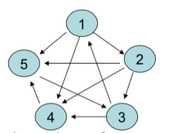
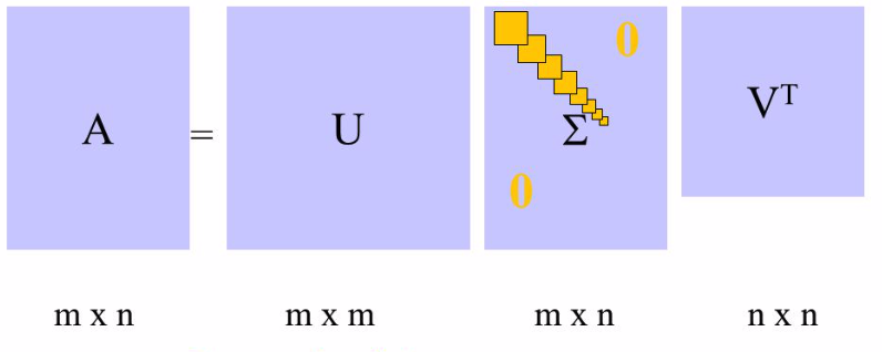
Bayesian Statistics and Computing

---

# Bayesian Statistics and Computing

## Lecture 15: Singular Value Decomposition

#### *Yanfei Kang | BSC | 2021 Spring*

---

# Why numerical linear algebra?

- Difference between linear algebra and **applied** linear algebra.

- Think about linear algebra in Statistics.

- In curve fitting.

- In image processing.

- In signal processing.

- etc.

- **We need to know numerical techniques!**

---
# What we will learn in this lecture

- Eigenanalysis

- SVD
    
---
class: inverse, center, middle
# Eigenanalysis

---
# Eigenanalysis

- In general, a matrix acts on a vector by changing both its magnitude and its direction.

- However, a matrix may act on certain vectors by changing only their magnitude, and leaving their direction unchanged (or reversing it).
    - these vectors are the eigenvectors of the matrix
    - the scaling factor is the eigenvalue.

---
# Eigenanalysis

- What if `$\mathbf{A}$` is not a square matrix?

- How to find its eigenvalues and eigenvectors?

- If `$\mathbf{A}$` is a real symmetric matrix
    - Only real eigenvalues
    - `$n$` distinct linearly independent eigenvectors
    - pairwise orthogonal
    - `$\mathbf{A = Q\Lambda Q^T}$`
    
- When `$A$` is diagonalisable?

- If a diagonalisation doesn't exist, there is always a triangularisation via Schur Decomposition: `$\mathbf{A = QSQ^T}$`.

- Let us revisit together the properties of eigenvalues and eigenvectors.

---
# What does eigenanalysis help to do?

- Let's try to understand what `$\mathbf{Ax} = \lambda \mathbf{x}$` is really asking.

- Can we find a pair of `$\lambda$` and `$\mathbf{x}$` such that when a matrix `$\mathbf{A}$` is applied to `$\mathbf{x}$`, it doesn't change the direction and just scales the vector?

- If we can find such a pair, then everytime we do something with `$\mathbf{Ax}$` in some mathematical operation, we can replace it with `$\lambda \mathbf{x}$`.

---
# What does eigenanalysis help to do?

- Consider `$\mathbf{A} = \left(\begin{array}{cc}5 & -1\\-2 & 4 \end{array}\right)$` and `$\mathbf{x} = \left(\begin{array}{c}1 \\-1 \end{array}\right)$`.

- What if we now want to calculate `$\mathbf{A^{20}x}$`?

- What if we now want to calculate `$\mathbf{A^{-1}x}$`?

---
# Advantages of eigenanalysis

- It enables us to replace a matrix with a scalar when we have the opportunity to change our coordinate system to the eigenvectors of a matrix.

- We can express any vector in terms of this new coordinate system.

- We can use the fact that `$\mathbf{Ax} = \lambda \mathbf{x}$` to simplify calculations.

---
# Application of Eigenanalysis: Google

---
# How to know page rank?

- How does the search engine know which pages are the most important?

- Google assigns a number to each individual page, expressing its importance.

- This number is known as the PageRank and is computed via the eigenvalue problem `$Aw = \lambda w$`, where `$A$` is based on the link structure of the Internet.

---
# Google's pagerank

- Suppose we have a set of webpages `$W$`, with `$|W|=n$` as the number of webpages.

- We define a connectivity (adjacency) matrix `$A$` as follows:
`$$A_{i j}:=\left\{\begin{array}{ll}
1 / N_{i} & \text{if Page } i \text{ links to  Page } j, \\
0 & \text { otherwise.}
\end{array}\right.$$`
where `$N_i$` is the number of outlinks on Page `$i$`.

- Typically `$A$` is huge (27.5 billion x 27.5 billion in 2011), but extremely sparse (lots of zero values)

---
# A small example

.pull-right[
The connectivity matrix is 
`$$A =\left(\begin{array}{lllll}
0 & 1/3 & 0 & 1/3 & 1/3 \\
0 & 0 & 1/3 & 1/3 & 1/3 \\
1/2 & 0 & 0 & 1/2 & 0 \\
0 & 0 & 0 & 0 & 1 \\
0 & 0 & 1 & 0 & 0
\end{array}\right)$$`
]

---
# A small example

- The underlying idea for PageRank: a page is important, if other important pages link to it.

- The ranking of page `$i$` is proportional to the weighted sum of the rankings of all pages that link to `$i$`: `$r_4 = \frac{1}{3}r_1 + \frac{1}{3}r_2 + \frac{1}{2}r_3$`.

- So this is a system of `$n = 5$` linear equations (please write it out).

- The ranking vector is treated like a probability of relevance, so we
need to then rescale so that `$\Sigma_{i=1}^n r_i = 1.$`

- Go to R and compute page ranks in this example.

---
# What you need to realise for now

- Finding the eigenvalues and eigenvectors of a massive matrix is computationally challenging though (don’t try to solve the characteristic polynomial!)

- And you will learn numerical techniques later.

---
# Further readings

[Google's pagerank](https://yanfei.site/docs/bsc/pagerank.pdf).

---
class: inverse, center, middle
# Singular Value Decomposition (SVD)

---
# Non-square matrices

- Recall that if the matrix A is square (real or complex) then a diagonalisation may exist.
    - This is clearly very useful for easy calculation of many important problems as we saw last week.
    - If a diagonalisation doesn't exist, then there is always a triangularisation via Schur Decomposition.
    
- But non-square matrices don’t have eigenvalues, so what can we do?

- You are about to learn the most useful diagonal decomposition that works for all matrices: Singular Value Decomposition.

---
#  Singular values

- Singular values are the square roots of the eigenvalues of `$A^TA$` which is square and symmetric.

-  `$u$` and `$v$` come in a pair for each
singular value `$\sigma$`, such that `$$A v = \sigma u.$$`

- `$u$` and `$v$` are eigenvectors of `$AA^T$` and `$A^TA$`, respectively.

---
#  Generalising Eigen-Decomposition

- Eigendecomposition involves only one eigenvector for each eigenvalue (including multiplicities), stored in an orthogonal matrix `$Q$`, with eigenvalues on the diagonal of the matrix `$\Lambda$`, so that `$A=Q\Lambda Q^T$`.

- We can generalise this now that we have singular vectors `$u$` and `$v$` for each singular value `$\sigma$`.

---
# Singular Value Decomposition (SVD)

For `$A \in \mathcal{R}^{m \times n}$`, there exists orthogonal matrices 
`$$U = [u_1, \cdots, u_m] \in \mathcal{R}^{m\times m}$$` and 
`$$V = [v_1, \cdots, v_n] \in \mathcal{R}^{n\times n}$$`
such that
`$$U^TAV = \Sigma = \text{diag}\{\sigma_1, \cdots, \sigma_p\} \in \mathcal{R}^{m\times n},$$`
with `$p = \min\{m, n\}$` and `$\sigma_1 \geq \dots \geq \sigma_p \geq 0$`.

Rearranging, we have `$$A = U\Sigma V^T$$`.

---
# SVD

Try `svd()` in R.

---
# Some properties of SVD

- `$\sigma_i$` are singular values of `$A$`.

- The non-zero singular values of `$A$` are the square roots of the non-zero eigenvalues of both `$A^TA$` and `$AA^T$`.

- The rank of a matrix is equal to the number of non-zero singular values.

- The condition number measures the degree of singularity of `$A^TA$`:
`$$\kappa = \frac{\text{max singular value}}{\text{min singular value}}.$$`
- **What is the relationship of SVD and PCA?**

---
# Applications of SVD

- In data compression, we start with a matrix A that contains perfect data, and we try to find a (lower-rank) approximation to the data that seeks to capture the principal elements of the data.
     - we sacrifice only the less important parts that don’t degrade data quality too much, in order to gain compression.
- In noise filtering, we start with a matrix A that contains imperfect data, and we try to find a (lower-rank) approximation to the data that seeks to capture the principal elements of the data.
     - we give up only the less important parts that are typically noise.
- So both these tasks are related, and rely on the SVD to find a suitable lower-ranked approximation to a matrix.

---
class: inverse, center, middle
# Matrix Approximation

---
# SVD components

Recall that the SVD of a matrix `$A$` in `$\mathcal{R}_{m\times n}$` decomposes the matrix into `$$A = U\Sigma V^T = \left(\begin{array}{cc}U_1 & U_2\end{array}\right) \left(\begin{array}{cc} D & \\& 0\end{array}\right) \left(\begin{array}{cc}V_1^T & V_2^T\end{array}\right) = U_1DV_1^T$$`
where `$D = \text{diag}\{\sigma_1, \cdots, \sigma_r\} \in \mathcal{R}^{r\times r}$` with `$\sigma_r > 0$` for `$r = \text{rank}(A)$`.

<center>
![](./figs/svd.png)

---
# Matrix Approximation

- `$A$` can also be expressed as a sum of outer products, with each sum being a rank 1 matrix of dimension `$m\times n$` 
`$$A = \Sigma_{i = 1}^r \sigma_i u_i v_i^T = \sigma_1 u_1 v_1^T + \cdots + \sigma_r u_r v_r^T.$$`

- We can truncate this sum when we feel that the singular values are so small that they are not contributing much.

---
class: inverse, center, middle
# Image Compression

---
# Image Compression

- Suppose we have a grayscale image (*128 x 128* pixels).
    - We can use a matrix to represent this image.
    
- If we have a colour image, it has three matrices, with the same size as the image. Each matrix represents a color value that comprises the RGB color scale.

- Each pixel is represented by an integer from 0-255.

- Next, we can decompose the matrix by SVD.

- By eliminating small singular values, we can approximate the matrix.
    - Choose the value of `$k$` for the low-rank approximation `$A_k$`.
    - Plotting the singular values might help identify where there is a noticeable drop in significance.
    
---
# Reconstructing approximated image

- Suppose we have chosen the value of `$k$` = number of singular values we wish to retain. - We can generate a new image matrix by expanding `$A$` using the SVD (first `$k$` singular values only).

- If you want to use colour images, do it for R, G, B matrices separately and then reassemble.

---
# Data compression

```r
library(jpeg)
ykang <- readJPEG("./figs/ykang.jpg")
r <- ykang[, , 1]
g <- ykang[, , 2]
b <- ykang[, , 3]
ykang.r.svd <- svd(r)
ykang.g.svd <- svd(g)
ykang.b.svd <- svd(b)
rgb.svds <- list(ykang.r.svd, ykang.g.svd, ykang.b.svd)
for (j in seq.int(4, 200, length.out = 8)) {
 a <- sapply(rgb.svds, function(i) {
 ykang.compress <- i$u[, 1:j] %*% diag(i$d[1:j]) %*% t(i$v[, 1:j])
 }, simplify = "array")
 writeJPEG(a, paste("./figs/", "ykang_svd_rank_", round(j, 0), ".jpg", sep = ""))
}
```

Here are four images with rank 286, 200, 116 and 32.

<img src="figs/ykang.jpg" width="200" /> 
 <img src="figs/ykang_svd_rank_200.jpg" width="200" /> 
 <img src="figs/ykang_svd_rank_116.jpg" width="200" />
 <img src="figs/ykang_svd_rank_32.jpg" width="200" />

]

---
class: inverse, center, middle
# Linear regression

---
# Linear regression

For a linear regression, 
`$$\mathbf{y} = \mathbf{X}\mathbf{\beta} + \mathbf{\varepsilon},~\mathbf{\epsilon}\sim N(0,\Sigma).$$`
what is its OLS solution?

---
#  Numerical Issues

- Numerically, there can be problems with solving for `$\mathbf{\beta}$` via the normal equations.
    - The inverse of `$X^TX$` might not exist
    - It is not computationally efficient to invert it for large dimensions
    - `$X^TX$` maybe ill-conditioned
    
- The SVD can help us by providing a numerically stable pseudo-inverse, and the opportunity to identify (through the singular values) any ill-conditioning.

---
# Pseudo-inverse

Recall that the SVD of a matrix `$A$` in `$\mathcal{R}_{m\times n}$` decomposes the matrix into `$$A = U\Sigma V^T = \left(\begin{array}{cc}U_1 & U_2\end{array}\right) \left(\begin{array}{cc}D & \\& 0\end{array}\right) \left(\begin{array}{cc}V_1^T & V_2^T\end{array}\right) = U_1DV_1^T$$`
where `$D = \text{diag}\{\alpha_1, \cdots, \alpha_r\} \in \mathcal{R}^{r\times r}$` with `$\sigma_r > 0$` for `$r = \text{rank}(A)$`.

- The pseudo-inverse, or generalised inverse, of `$A$` can always be calculated, even if 
`$A$` is not invertible.
`$$A^+ = V_1D^{-1}U_1^T$$`
- `$A^{+}$` is `$n \times m$`.

---
# Linear regression

For `$$\mathbf{y} = \mathbf{X}\mathbf{\beta} + \mathbf{\varepsilon},~\mathbf{\epsilon}\sim N(0,\Sigma),$$`
the solution is 
`$$\beta = X^{+}y = V_1D^{-1}U_1^T y = \Sigma_{i = 1}^r \frac{v_iu_i^Ty}{\sigma_i}.$$`
A small singular value means trouble. A lower rank approximation should be more reliable.